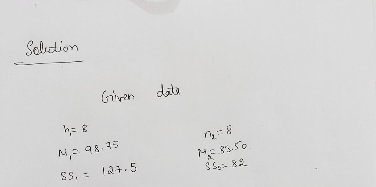
It was hypothesized that there will be a difference in average test score in chemistry class between high schoolers who watched Breaking Bad (G1) and high schoolers who did not watch Breaking Bad (G2). Calculate and use the appropriate statistical test to analyze the below. Alpha criteria is set at 0.01. Watched Breaking Bad 99 Did Not Watch Breaking Bad 90 82 85 82 86 79 91 98 97 94 86 92 83 93 81 n = 8 M = 93.75 SS = 127.5 n = 8 M = 83.50 SS = 82 Is this a one-tailed or two-tailed hypothesis? What is your degrees of freedom?
It was hypothesized that there will be a difference in average test score in chemistry class between high schoolers who watched Breaking Bad (G1) and high schoolers who did not watch Breaking Bad (G2). Calculate and use the appropriate statistical test to analyze the below. Alpha criteria is set at 0.01. Watched Breaking Bad 99 Did Not Watch Breaking Bad 90 82 85 82 86 79 91 98 97 94 86 92 83 93 81 n = 8 M = 93.75 SS = 127.5 n = 8 M = 83.50 SS = 82 Is this a one-tailed or two-tailed hypothesis? What is your degrees of freedom?

MATLAB: An Introduction with Applications
6th Edition
ISBN:9781119256830
Author:Amos Gilat
Publisher:Amos Gilat
Chapter1: Starting With Matlab
Section: Chapter Questions
Problem 1P

Related questions
Question

Transcribed Image Text:It was hypothesized that there will be a difference in average test score in chemistry class between high schoolers who watched Breaking Bad (G1) and high schoolers who did
not watch Breaking Bad (G2). Calculate and use the appropriate statistical test to analyze the below. Alpha criteria is set at 0.01.
Watched Breaking Bad
Did Not Watch Breaking Bad
86
99
90
79
91
94
82
86
98
92
85
83
97
93
82
81
n = 8
M = 93.75
n = 8
M = 83.50
SS = 82
SS = 127.5
%3D
%!
Is this a one-tailed or two-tailed hypothesis?
What is your degrees of freedom?
What is your effect size? Express to the nearest hundredths.

Transcribed Image Text:t Table
cum. prob
t so
0.50
t 3o
t s0
0.10
0.20
tas
t st
0.05
t 975
t g95
t 99
t 9995
one-tail
two-tails
0.25
0.20
0.15
0.025
0.01
0.005
0.001 0.0005
1.00
0.50
0.40
0.30
0.10
0.05
0.02
0.01
0.002
0.001
IP
0.000
1.000
1.376
1.963
3.078
1.886
1.638
1.533
6.314
12.71
31.82
6.965
63.66
9.925
318.31
22.327
10.215
7.173
636.62
31.599
0.000
0.816
1.061
1.386
2.920
2.353
2.132
4.303
3.182
0.000
0.765
0.978
1.250
4.541
5.841
12.924
4
5
0.000
0.741
0.941
1.190
2.776
3.747
4.604
8.610
6.869
5.959
0.000
0.727
0.920
1.156
1.134
1.476
2.015
2.571
3.365
3.143
4.032
3.707
5.893
0.000
0.000
0.718
0.906
1.440
1.943
1.895
2.447
5.208
4.785
4.501
7
8
9
10
11
12
13
14
15
16
17
18
19
20
0.711
0.896
1.119
1.415
2.365
2.998
3.499
3.355
5.408
0.000
0.706
0.889
1.108
1.397
1.860
2.306
2.896
5.041
0.000
0.703
0.883
1.100
1.383
1.372
1.363
1.833
2.262
2.821
3.250
4.297
4.144
4.025
4.781
0.000
0.879
0.700
0.697
1.093
1.812
2.228
2.764
2.718
3.169
4.587
4.437
0.000
0.876
1.088
1.796
2.201
3.106
3.055
0.000
0.695
0.694
0.873
1.083
1.356
1.782
2.179
2.681
3.930
4.318
0.000
0.000
0.000
0.870
0.868
1.079
1.350
1.771
2.160
3.852
3.787
3.733
3.686
3.646
3.610
3.579
3.552
2.650
3.012
4.221
0.692
1.076
1.345
1.761
2.145
2.624
4.140
4.073
4.015
3.965
2.977
0.691
0.866
0.865
1.074
1.341
2.131
1.753
1.746
2.947
2.921
2.602
0.000
0.690
1.071
1.337
2.120
2.583
0.000
0.689
0.688
0.863
1.069
1.333
1.740
2.110
2.567
2.898
0.000
0.862
1.067
1.330
1.328
1.325
1.734
2.101
2.093
2.086
2.552
2.878
3.927
3.883
3.850
3.819
3.792
3.768
3.745
3.725
0.000
0.688
0.687
0.861
1.066
1.064
1.729
2.539
2.861
0.000
0.860
1.725
2.528
2.845
21
0.000
0.686
0.859
1.063
1.323
1.721
2.080
2.518
2.831
3.527
3.505
3.485
3.467
22
23
24
25
26
27
28
29
30
40
60
80
100
1000
0.000
0.686
0.858
1.061
1.321
1.717
2.074
2.508
2.819
0.000
0.685
0.858
1.060
1.319
1.714
2.069
2.500
2.807
0.000
0.685
0.857
1.059
1.318
1.711
2.064
2.492
2.797
0.000
0.684
0.856
1.058
1.316
1.708
2.060
2.485
2.787
3.450
0.000
0.684
1.706
1.703
0.856
1.058
1.315
2.056
2.479
2.779
3.435
3.707
0.000
0.000
0.684
0.855
1.057
1.314
2.052
2.473
2.771
3.421
3.690
0.683
0.855
1.056
1.701
1.313
1.311
2.048
2.467
2.763
2.756
3.408
3.674
0.000
0.683
0.854
1.055
1.699
2.045
2.462
3.396
3.659
0.000
0.683
0.854
1.055
1.050
1.310
1.697
2.042
2.457
2.750
3.385
3.307
3.232
3.195
3.174
3.646
0.000
0.681
0.851
1.303
1.684
2.021
2.423
2.704
3.551
0.000
0.679
0.848
1.045
1.296
1.671
2.000
2.390
2.660
2.639
3.460
0.000
0.678
0.846
1.043
1.292
1.664
1.990
2.374
3.416
0.000
0.677
0.845
1.042
1.290
1.660
1.984
2.364
2.626
3.390
0.000
0.675
0.842
1.037
1.282
1.646
1.962
2.330
2.581
3.098
3.300
0.000
0.674
0.842
1.036
1.282
1.645
1.960
2.326
2.576
3.090
3.291
60%
80%
95%
Confidence Level
0%
50%
70%
90%
98%
99% 99.8% 99.9%
123 456 789O
Expert Solution
Step 1

Step by step
Solved in 2 steps with 2 images

Recommended textbooks for you
MATLAB: An Introduction with Applications
Statistics
ISBN:
9781119256830
Author:
Amos Gilat
Publisher:
John Wiley & Sons Inc

Probability and Statistics for Engineering and th…
Statistics
ISBN:
9781305251809
Author:
Jay L. Devore
Publisher:
Cengage Learning

Statistics for The Behavioral Sciences (MindTap C…
Statistics
ISBN:
9781305504912
Author:
Frederick J Gravetter, Larry B. Wallnau
Publisher:
Cengage Learning
MATLAB: An Introduction with Applications
Statistics
ISBN:
9781119256830
Author:
Amos Gilat
Publisher:
John Wiley & Sons Inc
Probability and Statistics for Engineering and th…
Statistics
ISBN:
9781305251809
Author:
Jay L. Devore
Publisher:
Cengage Learning
Statistics for The Behavioral Sciences (MindTap C…
Statistics
ISBN:
9781305504912
Author:
Frederick J Gravetter, Larry B. Wallnau
Publisher:
Cengage Learning

Elementary Statistics: Picturing the World (7th E…
Statistics
ISBN:
9780134683416
Author:
Ron Larson, Betsy Farber
Publisher:
PEARSON

The Basic Practice of Statistics
Statistics
ISBN:
9781319042578
Author:
David S. Moore, William I. Notz, Michael A. Fligner
Publisher:
W. H. Freeman

Introduction to the Practice of Statistics
Statistics
ISBN:
9781319013387
Author:
David S. Moore, George P. McCabe, Bruce A. Craig
Publisher:
W. H. Freeman