To test H9: u= 105 versus H,: u# 105 a simple random sample of size n= 35 is obtained. Complete parts a through e below. Click here to view the t-Distribution Area in Right Tail. (a) Does the population have to be normally distributed to test this hypothesis? Why? A. No, because n2 30. O B. Yes, because n2 30. OC. No, because the test is two-tailed. O D. Yes, because the sample is random. (b) If x= 102.0 and s= 5.8, compute the test statistic. The test statistic is to (Round to two decimal places as needed.)

Glencoe Algebra 1, Student Edition, 9780079039897, 0079039898, 2018
18th Edition
ISBN:9780079039897
Author:Carter
Publisher:Carter
Chapter10: Statistics
Section10.1: Measures Of Center
Problem 9PPS
icon
Related questions
icon
Concept explainers
Question
To test Ho: u= 105 versus H,: µ 105 a simple random sample of size n = 35 is obtained. Complete parts a through e below.
Click here to view the t-Distribution Area in Right Tail.
(a) Does the population have to be normally distributed to test this hypothesis? Why?
A. No, because n2 30.
O B. Yes, because n2 30.
O C. No, because the test is two-tailed.
O D. Yes, because the sample is random.
(b) lf x= 102.0 and s = 5.8, compute the test statistic.
The test statistic is to =| (Round to two decimal places as needed.)
Transcribed Image Text:To test Ho: u= 105 versus H,: µ 105 a simple random sample of size n = 35 is obtained. Complete parts a through e below. Click here to view the t-Distribution Area in Right Tail. (a) Does the population have to be normally distributed to test this hypothesis? Why? A. No, because n2 30. O B. Yes, because n2 30. O C. No, because the test is two-tailed. O D. Yes, because the sample is random. (b) lf x= 102.0 and s = 5.8, compute the test statistic. The test statistic is to =| (Round to two decimal places as needed.)
Expert Solution
trending now

Trending now

This is a popular solution!

steps

Step by step

Solved in 2 steps

Blurred answer
Follow-up Questions
Read through expert solutions to related follow-up questions below.
Follow-up Question
(e) If the researcher decides to test this hypothesis at the x = 0.05 level of significance, will the researcher reject the
null hypothesis?
Yes
O No
Transcribed Image Text:(e) If the researcher decides to test this hypothesis at the x = 0.05 level of significance, will the researcher reject the null hypothesis? Yes O No
Solution
Bartleby Expert
SEE SOLUTION
Follow-up Question
Interpret the P-value. Choose the correct answer below.
A. If 100 random samples of size n = 35 are obtained, about 4 samples are expected to result in a mean as extreme or more extreme than the one observed if μ = 105.
B. If 1000 random samples of size n = 35 are obtained, about 4 samples are expected to result in a mean as extreme or more extreme than the one observed if μ = 105.
C. If 1000 random samples of size n = 35 are obtained, about 4 samples are expected to result in a mean as extreme or more extreme than the one observed if μ = 102.0.
D. If 1000 random samples of size n = 35 are obtained, about 10 samples are expected to result in a mean as extreme or more extreme than the one observed if μ = 105.
Transcribed Image Text:Interpret the P-value. Choose the correct answer below. A. If 100 random samples of size n = 35 are obtained, about 4 samples are expected to result in a mean as extreme or more extreme than the one observed if μ = 105. B. If 1000 random samples of size n = 35 are obtained, about 4 samples are expected to result in a mean as extreme or more extreme than the one observed if μ = 105. C. If 1000 random samples of size n = 35 are obtained, about 4 samples are expected to result in a mean as extreme or more extreme than the one observed if μ = 102.0. D. If 1000 random samples of size n = 35 are obtained, about 10 samples are expected to result in a mean as extreme or more extreme than the one observed if μ = 105.
Solution
Bartleby Expert
SEE SOLUTION
Follow-up Question
Interpret the P-value. Choose the correct answer below.
A. If 100 random samples of size n = 35 are obtained, about 4 samples are expected to result in a mean as extreme or more extreme than the one observed if μ = 105.
B. If 1000 random samples of size n = 35 are obtained, about 4 samples are expected to result in a mean as extreme or more extreme than the one observed if μ = 105.
C. If 1000 random samples of size n = 35 are obtained, about 4 samples are expected to result in a mean as extreme or more extreme than the one observed if μ
D. If 1000 random samples of size n = 35 are obtained, about 10 samples are expected to result in a mean as extreme or more extreme than the one observed if
= 102.0.
= 105.
Transcribed Image Text:Interpret the P-value. Choose the correct answer below. A. If 100 random samples of size n = 35 are obtained, about 4 samples are expected to result in a mean as extreme or more extreme than the one observed if μ = 105. B. If 1000 random samples of size n = 35 are obtained, about 4 samples are expected to result in a mean as extreme or more extreme than the one observed if μ = 105. C. If 1000 random samples of size n = 35 are obtained, about 4 samples are expected to result in a mean as extreme or more extreme than the one observed if μ D. If 1000 random samples of size n = 35 are obtained, about 10 samples are expected to result in a mean as extreme or more extreme than the one observed if = 102.0. = 105.
Solution
Bartleby Expert
SEE SOLUTION
Follow-up Question
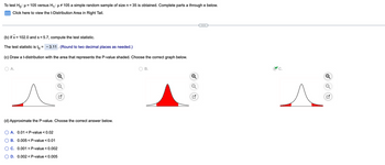
To test Ho: μ = 105 versus H₁: μ‡ 105 a simple random sample of size n = 35 is obtained. Complete parts a through e below.
Click here to view the t-Distribution Area in Right Tail.
(b) If x= 102.0 and s=5.7, compute the test statistic.
=
The test statistic is to
(c) Draw a t-distribution with the area that represents the P-value shaded. Choose the correct graph below.
O A.
-3.11. (Round to two decimal places as needed.)
(d) Approximate the P-value. Choose the correct answer below.
A. 0.01 < P-value < 0.02
B. 0.005 < P-value < 0.01
C. 0.001 < P-value < 0.002
D. 0.002 < P-value < 0.005
B.
W
17
Transcribed Image Text:To test Ho: μ = 105 versus H₁: μ‡ 105 a simple random sample of size n = 35 is obtained. Complete parts a through e below. Click here to view the t-Distribution Area in Right Tail. (b) If x= 102.0 and s=5.7, compute the test statistic. = The test statistic is to (c) Draw a t-distribution with the area that represents the P-value shaded. Choose the correct graph below. O A. -3.11. (Round to two decimal places as needed.) (d) Approximate the P-value. Choose the correct answer below. A. 0.01 < P-value < 0.02 B. 0.005 < P-value < 0.01 C. 0.001 < P-value < 0.002 D. 0.002 < P-value < 0.005 B. W 17
Solution
Bartleby Expert
SEE SOLUTION
Follow-up Question
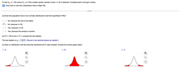
To test \( H_0: \mu = 105 \) versus \( H_1: \mu \neq 105 \), a simple random sample of size \( n = 35 \) is obtained. Complete parts a through e below.

(a) Does the population have to be normally distributed to test this hypothesis? Why?  
- A. No, because the test is two-tailed.  
- B. No, because \( n \geq 30 \). *(Correct)*  
- C. Yes, because \( n \geq 30 \).  
- D. Yes, because the sample is random.  

(b) If \( \bar{x} = 102.0 \) and \( s = 5.7 \), compute the test statistic.  
The test statistic is \( t_0 = -3.11 \). (Round to two decimal places as needed.)

(c) Draw a t-distribution with the area that represents the P-value shaded. Choose the correct graph below.  
- Option A: Graph with shaded left tail.  
- Option B: Graph with shaded center area.  
- Option C: Graph with shaded tails on both ends. *(Correct)*  

Explanation of Graphs:  
- **Option A** shows a normal distribution curve with shading in the left tail, indicating a one-tailed test.  
- **Option B** displays a distribution with shading in the center, which would not usually represent a P-value.  
- **Option C** illustrates two tails shaded on both ends of a normal distribution curve, properly representing a two-tailed test for the given hypothesis.
Transcribed Image Text:To test \( H_0: \mu = 105 \) versus \( H_1: \mu \neq 105 \), a simple random sample of size \( n = 35 \) is obtained. Complete parts a through e below. (a) Does the population have to be normally distributed to test this hypothesis? Why? - A. No, because the test is two-tailed. - B. No, because \( n \geq 30 \). *(Correct)* - C. Yes, because \( n \geq 30 \). - D. Yes, because the sample is random. (b) If \( \bar{x} = 102.0 \) and \( s = 5.7 \), compute the test statistic. The test statistic is \( t_0 = -3.11 \). (Round to two decimal places as needed.) (c) Draw a t-distribution with the area that represents the P-value shaded. Choose the correct graph below. - Option A: Graph with shaded left tail. - Option B: Graph with shaded center area. - Option C: Graph with shaded tails on both ends. *(Correct)* Explanation of Graphs: - **Option A** shows a normal distribution curve with shading in the left tail, indicating a one-tailed test. - **Option B** displays a distribution with shading in the center, which would not usually represent a P-value. - **Option C** illustrates two tails shaded on both ends of a normal distribution curve, properly representing a two-tailed test for the given hypothesis.
Solution
Bartleby Expert
SEE SOLUTION
Follow-up Question
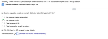
To test \( H_0: \mu = 105 \) versus \( H_1: \mu \neq 105 \), a simple random sample of size \( n = 35 \) is obtained. Complete parts a through b below.

---

(a) Does the population have to be normally distributed to test this hypothesis? Why?

- A. No, because the test is two-tailed.
- B. No, because \( n \geq 30 \). (Correct)
- C. Yes, because \( n \geq 30 \).
- D. Yes, because the sample is random.

(b) If \( \bar{x} = 102.0 \) and \( s = 5.7 \), compute the test statistic.

The test statistic is \( t_0 = \_ \_ \). (Round to two decimal places as needed.)
Transcribed Image Text:To test \( H_0: \mu = 105 \) versus \( H_1: \mu \neq 105 \), a simple random sample of size \( n = 35 \) is obtained. Complete parts a through b below. --- (a) Does the population have to be normally distributed to test this hypothesis? Why? - A. No, because the test is two-tailed. - B. No, because \( n \geq 30 \). (Correct) - C. Yes, because \( n \geq 30 \). - D. Yes, because the sample is random. (b) If \( \bar{x} = 102.0 \) and \( s = 5.7 \), compute the test statistic. The test statistic is \( t_0 = \_ \_ \). (Round to two decimal places as needed.)
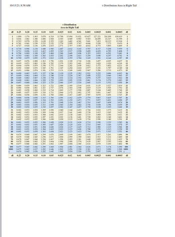
# t-Distribution: Area in Right Tail

This table displays the critical values of the t-distribution for different degrees of freedom (df) and the area in the right tail. It is used in statistical hypothesis testing, particularly for small sample sizes when the population standard deviation is unknown.

## Table Layout
- **Columns**: These represent the tail probabilities (areas) from 0.25 to 0.0005.
- **Rows**: These represent the degrees of freedom (df), ranging from 1 to 1000.

## Explanation of Table Content
For each combination of degrees of freedom and tail probability, the table provides the critical value of the t-distribution. This critical value is the t-score that separates the rightmost tail area from the rest of the distribution. The top section of the table illustrates values for df ranging from 1 to 20. The second section continues from df 21 to 40, and subsequent sections display values for selected degrees of freedom up to 1000.

### Example:
- At 10 degrees of freedom and an area of 0.05 in the right tail, the critical value is 1.812.
- For 30 degrees of freedom with an area of 0.01, the critical value is 2.457.

This table is essential for determining the threshold at which you would reject the null hypothesis in t-tests, ensuring accurate statistical analysis.
Transcribed Image Text:# t-Distribution: Area in Right Tail This table displays the critical values of the t-distribution for different degrees of freedom (df) and the area in the right tail. It is used in statistical hypothesis testing, particularly for small sample sizes when the population standard deviation is unknown. ## Table Layout - **Columns**: These represent the tail probabilities (areas) from 0.25 to 0.0005. - **Rows**: These represent the degrees of freedom (df), ranging from 1 to 1000. ## Explanation of Table Content For each combination of degrees of freedom and tail probability, the table provides the critical value of the t-distribution. This critical value is the t-score that separates the rightmost tail area from the rest of the distribution. The top section of the table illustrates values for df ranging from 1 to 20. The second section continues from df 21 to 40, and subsequent sections display values for selected degrees of freedom up to 1000. ### Example: - At 10 degrees of freedom and an area of 0.05 in the right tail, the critical value is 1.812. - For 30 degrees of freedom with an area of 0.01, the critical value is 2.457. This table is essential for determining the threshold at which you would reject the null hypothesis in t-tests, ensuring accurate statistical analysis.
Solution
Bartleby Expert
SEE SOLUTION
Knowledge Booster
Continuous Probability Distribution
Learn more about
Need a deep-dive on the concept behind this application? Look no further. Learn more about this topic, statistics and related others by exploring similar questions and additional content below.
Recommended textbooks for you
Glencoe Algebra 1, Student Edition, 9780079039897…
Algebra
ISBN:
9780079039897
Author:
Carter
Publisher:
McGraw Hill