Illustrate the instantaneous frequency for the following FM modulated waveforms: kHz S fm (t) = A cos[2πft+2nk, fm (t)dt], f = 100 MHz, k, = 10: Volt a) with m (t) = Σm rect k=1 {rect (¹-KT) m² = {-1,1} b) with m (0)= Emreal-AT) met-2,2} rect (¹~KT) m = {-4,4} c) with m (t)= Σm, rect( kul
Illustrate the instantaneous frequency for the following FM modulated waveforms: kHz S fm (t) = A cos[2πft+2nk, fm (t)dt], f = 100 MHz, k, = 10: Volt a) with m (t) = Σm rect k=1 {rect (¹-KT) m² = {-1,1} b) with m (0)= Emreal-AT) met-2,2} rect (¹~KT) m = {-4,4} c) with m (t)= Σm, rect( kul

Introductory Circuit Analysis (13th Edition)
13th Edition
ISBN:9780133923605
Author:Robert L. Boylestad
Publisher:Robert L. Boylestad
Chapter1: Introduction
Section: Chapter Questions
Problem 1P: Visit your local library (at school or home) and describe the extent to which it provides literature...

Related questions
Question
I need help with this problem. Steps of what's happening would be helpful please and thank you!
![The text describes the instantaneous frequency of frequency-modulated (FM) waveforms. The modulation index and signal are expressed using different values for \( m(t) \). Here's a transcription and explanation suitable for an educational website:
---
**Illustration of Instantaneous Frequency for FM Modulated Waveforms**
The FM signal is given by:
\[
s_{fm}(t) = A_c \cos\left[2\pi f_c t + 2\pi k_f \int_0^t m(\tau) d\tau \right]
\]
Where:
- \( f_c = 100 \, \text{MHz} \) is the carrier frequency.
- \( k_f = 10 \, \text{kHz/Volt} \) is the frequency sensitivity.
The modulation function \( m(t) \) is described for different cases:
**Case a)**
\[ m(t) = \sum_{k=1}^{N} m_k \, \text{rect}\left(\frac{t-kT}{T}\right), \quad m_k \in \{-1, 1\} \]
**Case b)**
\[ m(t) = \sum_{k=1}^{N} m_k \, \text{rect}\left(\frac{t-kT}{T}\right), \quad m_k \in \{-2, 2\} \]
**Case c)**
\[ m(t) = \sum_{k=1}^{N} m_k \, \text{rect}\left(\frac{t-kT}{T}\right), \quad m_k \in \{-4, 4\} \]
- The term \( \text{rect}\left(\frac{t-kT}{T}\right) \) represents a rectangular pulse centered at \( kT \) with duration \( T \).
- \( m_k \) are the amplitudes that change in each case, affecting the modulation depth.
**Explanation:**
- In Case a, \( m(t) \) switches between -1 and 1, creating a frequency deviation based on these values.
- In Case b, \( m(t) \) switches between -2 and 2, leading to larger frequency deviations.
- In Case c, \( m(t) \) switches between -4 and 4, resulting in even greater frequency deviations.
Each case illustrates how varying \( m_k \) values influence the instantaneous](/v2/_next/image?url=https%3A%2F%2Fcontent.bartleby.com%2Fqna-images%2Fquestion%2F2a39407e-8b6e-45ca-91f9-5cf33a72fdc4%2F3237fed0-3b21-4537-acf3-4a93706b54b1%2F5sw3ofo_processed.jpeg&w=3840&q=75)
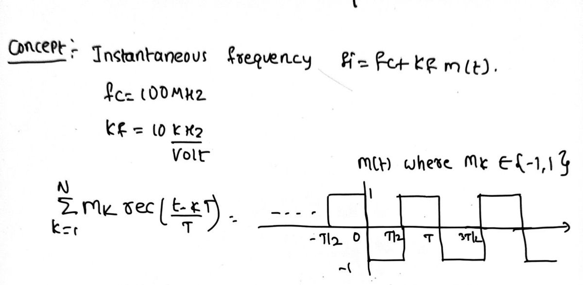
Transcribed Image Text:The text describes the instantaneous frequency of frequency-modulated (FM) waveforms. The modulation index and signal are expressed using different values for \( m(t) \). Here's a transcription and explanation suitable for an educational website:
---
**Illustration of Instantaneous Frequency for FM Modulated Waveforms**
The FM signal is given by:
\[
s_{fm}(t) = A_c \cos\left[2\pi f_c t + 2\pi k_f \int_0^t m(\tau) d\tau \right]
\]
Where:
- \( f_c = 100 \, \text{MHz} \) is the carrier frequency.
- \( k_f = 10 \, \text{kHz/Volt} \) is the frequency sensitivity.
The modulation function \( m(t) \) is described for different cases:
**Case a)**
\[ m(t) = \sum_{k=1}^{N} m_k \, \text{rect}\left(\frac{t-kT}{T}\right), \quad m_k \in \{-1, 1\} \]
**Case b)**
\[ m(t) = \sum_{k=1}^{N} m_k \, \text{rect}\left(\frac{t-kT}{T}\right), \quad m_k \in \{-2, 2\} \]
**Case c)**
\[ m(t) = \sum_{k=1}^{N} m_k \, \text{rect}\left(\frac{t-kT}{T}\right), \quad m_k \in \{-4, 4\} \]
- The term \( \text{rect}\left(\frac{t-kT}{T}\right) \) represents a rectangular pulse centered at \( kT \) with duration \( T \).
- \( m_k \) are the amplitudes that change in each case, affecting the modulation depth.
**Explanation:**
- In Case a, \( m(t) \) switches between -1 and 1, creating a frequency deviation based on these values.
- In Case b, \( m(t) \) switches between -2 and 2, leading to larger frequency deviations.
- In Case c, \( m(t) \) switches between -4 and 4, resulting in even greater frequency deviations.
Each case illustrates how varying \( m_k \) values influence the instantaneous
Expert Solution
Step 1

Step by step
Solved in 2 steps with 2 images

Knowledge Booster


Learn more about
Need a deep-dive on the concept behind this application? Look no further. Learn more about this topic, electrical-engineering and related others by exploring similar questions and additional content below.Recommended textbooks for you
Introductory Circuit Analysis (13th Edition)
Electrical Engineering
ISBN:
9780133923605
Author:
Robert L. Boylestad
Publisher:
PEARSON

Delmar's Standard Textbook Of Electricity
Electrical Engineering
ISBN:
9781337900348
Author:
Stephen L. Herman
Publisher:
Cengage Learning

Programmable Logic Controllers
Electrical Engineering
ISBN:
9780073373843
Author:
Frank D. Petruzella
Publisher:
McGraw-Hill Education
Introductory Circuit Analysis (13th Edition)
Electrical Engineering
ISBN:
9780133923605
Author:
Robert L. Boylestad
Publisher:
PEARSON
Delmar's Standard Textbook Of Electricity
Electrical Engineering
ISBN:
9781337900348
Author:
Stephen L. Herman
Publisher:
Cengage Learning
Programmable Logic Controllers
Electrical Engineering
ISBN:
9780073373843
Author:
Frank D. Petruzella
Publisher:
McGraw-Hill Education

Fundamentals of Electric Circuits
Electrical Engineering
ISBN:
9780078028229
Author:
Charles K Alexander, Matthew Sadiku
Publisher:
McGraw-Hill Education

Electric Circuits. (11th Edition)
Electrical Engineering
ISBN:
9780134746968
Author:
James W. Nilsson, Susan Riedel
Publisher:
PEARSON

Engineering Electromagnetics
Electrical Engineering
ISBN:
9780078028151
Author:
Hayt, William H. (william Hart), Jr, BUCK, John A.
Publisher:
Mcgraw-hill Education,