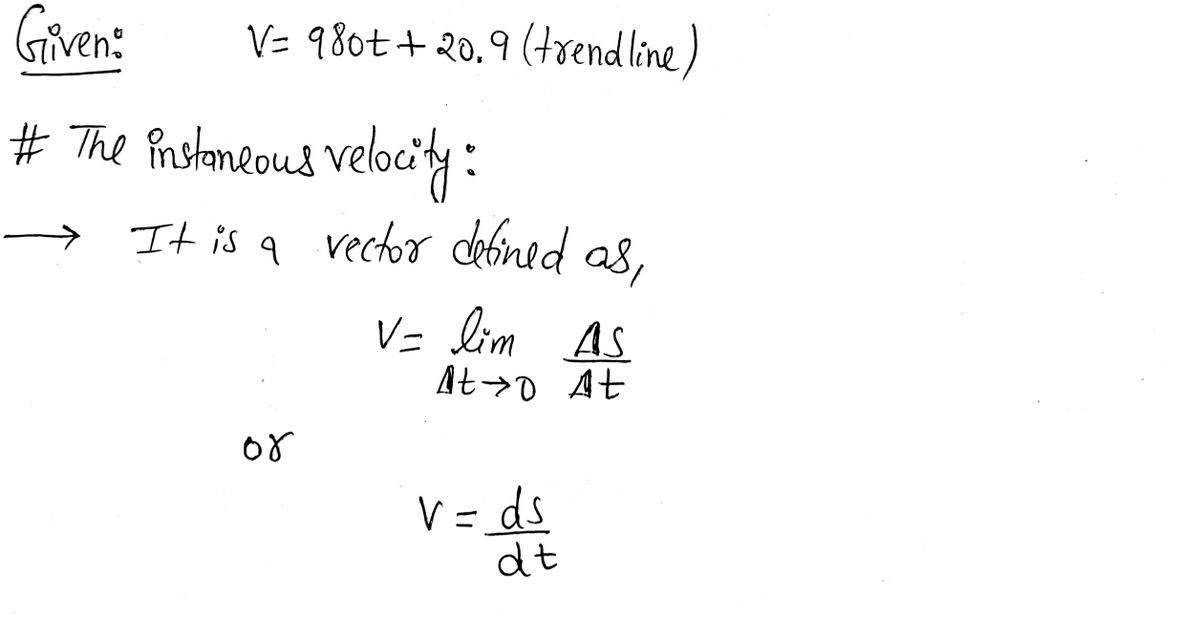
How do you calculate the instantaneous velocity from a velocity vs time graph?Eg. From the image below, Calculate the instantaneous velocity of V(4) at t(4),etc. The graph titled "V(ave) vs. t" displays the relationship between average velocity (V(ave)) and time (t). The horizontal axis represents time (t) in seconds, ranging from 0.1 to 0.4. The vertical axis represents average velocity (V(ave)), with values ranging from 0 to 500.The data points on the graph are plotted at four different times:1. At t = 0.1, V(ave) is 122.1.2. At t = 0.2, V(ave) is 213.7.3. At t = 0.3, V(ave) is 311.7.4. At t = 0.4, V(ave) is 416.2.These points have been connected with a straight line, indicating a linear relationship between average velocity and time. The line of best fit is described by the equation: V(ave) = 980*t + 20.9, where 980 is the slope and 20.9 is the y-intercept.This graph is useful in illustrating how average velocity increases linearly over time.

Answered: Image /qna-images/answer/a02f6f1d-2c8d-45d7-b2fe-b9f3c78ec216.jpg

Answered: How do you calculate the instantaneous…

How do you calculate the instantaneous velocity from a velocity vs time graph? Eg. From the image below, Calculate the instantaneous velocity of V(4) at t(4),etc.

Elements Of Electromagnetics

7th Edition

ISBN:9780190698614

Author:Sadiku, Matthew N. O.

Publisher:Sadiku, Matthew N. O.

ChapterMA: Math Assessment

Section: Chapter Questions

Problem 1.1MA

See similar textbooks

Similar questions

1 Overview In this project, you'll use several robot datasets for estimation and you will implement a Kalman Filter (KF) for state estimation. Consider the vehicle depicted in Fig. 1 with m = 0.5, k = 3.5, b = 2. The position s and velocity v represent the state x of the system and the input ƒ (t) is the force often denoted with u. F b m Figure 1: Robot cart 0 s(t) f(t) 1. Write the system in state space form and consider additive Gaussian white noise to the model n N (0, Q). Discretize the system state space form using Euler approach (30 points).
Look at the below system. Using either the conservation of energy method or Lagrange's method, solve for the governing equation of motion for the system. Put a box around your final answer. Also, put a box around your equations for the potential and kinetic energy of the system. Assume the system's springs are initially unstretched (i.e., assume that there is no gravity until t = 0 [s]). K₁ Î E K₂ X
i need the answer quickly
As shown in the following figure, vortices are shed from the rear of a bluff cylinder placed across a flow. The vortices alternately leave the top and bottom of the cylinder, causing an alternating force normal to the freestream velocity. The vortex shedding frequency, f, depends on the fluid density p, width of the cylinder d, freestream velocity V, and fluid viscosity u. (a) Use Buckingham Pi Theorem to develop a functional relationship for f. Use M, L, t as the primary dimensional. Use p, V, and d as the repeating parameters. (b) Vortex shedding occurs in standard air on two cylinders with a diameter ratio of 2. Determine the velocity ratio for dynamic similarity, and the ratio of vortex shedding frequencies. -Vortices V
The Laws of Physics are written for a Lagrangian system, a well-defined system which we follow around – we will refer to this as a control system (CSys). For our engineering problems we are more interested in an Eulerian system where we have a fixed control volume, CV, (like a pipe or a room) and matter can flow into or out of the CV. We previously derived the material or substantial derivative which is the differential transformation for properties which are functions of x,y,z, t. We now introduce the Reynold’s Transport Theorem (RTT) which gives the transformation for a macroscopic finite size CV. At any instant in time the material inside a control volume can be identified as a control System and we could then follow this System as it leaves the control volume and flows along streamlines by a Lagrangian analysis. RTT:DBsys/Dt = ∂/∂t ʃCV (ρb dVol) + ʃCS ρbV•n dA; uses the RTT to apply the laws for conservation of mass, momentum (Newton's Law), and energy (1st Law of…
Please ASAP: (image provided) a) Create a function to solve a projectile problem where you are given initial x and y velocity, and the initial and final y position (inputs). You would like to use this function to find the final x and y velocity (outputs). This function will be used in the solution of the following problem. b) In the figure below, belt A moves with a constant velocity of 5 ft/s, and discharges sand onto belt B as shown. Assume that the angle of belt B is 15 degrees as shown. Write a MATLAB program to determine the required velocity of belt B if the relative velocity with which the sand hits belt B is (a) vertical, and (b) as small as possible. For part (b), use MATLAB to create a plot of the velocity of the sand relative to belt B, as a function of the velocity of belt B. Verify (either by hand, or by using MATLAB) that the minimum shown in this plot corresponds to the point at which the velocity of the sand relative to belt B is perpendicular to the velocity of…
The Laws of Physics are written for a Lagrangian system, a well-defined system which we follow around – we will refer to this as a control system (CSys). For our engineering problems we are more interested in an Eulerian system where we have a fixed control volume, CV, (like a pipe or a room) and matter can flow into or out of the CV. We previously derived the material or substantial derivative which is the differential transformation for properties which are functions of x,y,z, t. We now introduce the Reynold’s Transport Theorem (RTT) which gives the transformation for a macroscopic finite size CV. At any instant in time the material inside a control volume can be identified as a control System and we could then follow this System as it leaves the control volume and flows along streamlines by a Lagrangian analysis. RTT:DBsys/Dt = ∂/∂t ʃCV (ρb dVol) + ʃCS ρbV•n dA; uses the RTT to apply the laws for conservation of mass, momentum (Newton's Law), and energy (1st Law of…
PLS DO FAST 2 THUMBS UP WILL BE GIVEN THANK U MAKE SURE NOT TO COPY FEOM ELSE WHERE THEY ARE WRONG THX
A projectile is launched with a velocity of 100 m/s at an angle of 30° above the horizontal. Create a Simulink model to solve the projectile's equations of motion, where x and y are the horizontal and vertical displacements of the projectile. X=0 x(0) = 100 cos 30º x(0)=0 ÿ=-g y(0)=0 y(0)=100 sin 30º Use the model to plot the projectile's trajectory y versus x for 0≤t≤10 s.
As we learned, Bernoulli's equation is not to be used in many situations. Let's say you are examining changes between two points in a flow. Which ONE of these scenarios could you appropriately use Bernoulli's equation on? O A turbine is situated between the two points There are large changes in kinetic energy between the two points The mass flow rate between the two points changes with time There are large changes in density between the two points There are large viscous losses between the two points QUESTION 10 A 12 cm diameter jet of air strikes a plate positioned normal to the flow, with all air deflected away parallel to the plate. If the air flows at a speed of 20 m/s, what is the force needed to held the plate in place? Do not use a linear momentum correction factor. O 0.272 N 10.9 N 4510 N 5.45 N 0.340 N
Here we have a very simple one dimensional model of a stroke rehabili- tation patient supported by a robot. Often, when you have a controlled electromechanical system like a robot and a human working together, you want to separate them by a compliant mechanism (spring with stiffness k) so that the robot has some "give". Otherwise, if there are errors in the control of the robot it can be very uncomfortable for a patient. The spring has zero force when x, = xp = 0. The patient provides viscous damping with damping Xp coefficient c. Fp + C Patient mp k Xp Robot Arm Xr Figure 2: Schematic diagram of a very simplified model of a patient pushing against a robot. The robot supports the patient via a spring for safety. In this case we want to eventually determine the force that the patient is exerting on the robot as a function of time, so we'll do some steps towards that goal. Your tasks: A Draw the free body diagram for the patient mass (mass mp). B Write the equations of motion for the…
4. Fluid Dynamics: Blood in a new pediatric blood cannula can be described by Equation 1 below. We assume that flow conditions are steady (time independent), fully developed (fluid layers moving consistently), with laminar flow properties (no mixing or rotational fluid dynamic properties). This fluid flow is often referred to as Poiseuille flow. The figure below illustrates the concept of Poiseuille flow and the characteristic parabolic velocity distribution. X 154 AL The governing fluid momentum equation in the x-flow direction is as follows: nd dv ΔΡ 74(*)= [1] r dr dr AL is the fluid viscosity, r refers to the radial position, and AP/AL signifies the where v corresponds to the velocity, imposed pressure gradient driving flow. a. Integrated the differential equation to find v(r). Using the following boundary conditions, determine the expressions for the constants of integration in the solution to part a) and the final velocity distribution equation (parabolic shape): v must be…