Draw the graph for the following probability: Between 1.4 and 2.6 Shade: Right of a value Click and drag the arrows to adjust the values.
Draw the graph for the following probability: Between 1.4 and 2.6 Shade: Right of a value Click and drag the arrows to adjust the values.

MATLAB: An Introduction with Applications
6th Edition
ISBN:9781119256830
Author:Amos Gilat
Publisher:Amos Gilat
Chapter1: Starting With Matlab
Section: Chapter Questions
Problem 1P

Related questions

Concept explainers
Contingency Table
A contingency table can be defined as the visual representation of the relationship between two or more categorical variables that can be evaluated and registered. It is a categorical version of the scatterplot, which is used to investigate the linear relationship between two variables. A contingency table is indeed a type of frequency distribution table that displays two variables at the same time.
Binomial Distribution
Binomial is an algebraic expression of the sum or the difference of two terms. Before knowing about binomial distribution, we must know about the binomial theorem.
Topic Video
Question

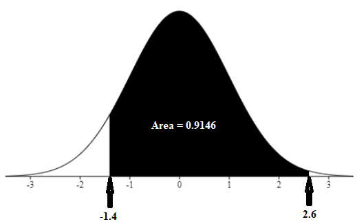
Transcribed Image Text:**Probability Graph Exploration**
To better understand probability distributions and shading under the normal distribution curve, we present the following example.
**Task: Draw the graph for the following probability: Between -1.4 and 2.6**
1. **Shade Option**:
- Select "Right of a value" to determine the area under the curve.
- You can adjust this by clicking and dragging the arrows to set the desired range.
2. **Graph Explanation**:
- The graph illustrates a normal distribution curve.
- The shading represents the area between -1.4 and 2.6 on the x-axis.
- The x-axis is marked with values ranging from -4 to 4, while the y-axis represents the probability density.
3. **Formula**:
- P(-1.4 < z < 2.6) is displayed as an input for further calculations.
4. **Submit Your Analysis**:
- After adjusting the shaded area, you can submit this configuration for analysis by clicking on the "Submit Question" button.
This exercise helps visualize how probabilities between two points can be represented graphically and helps in understanding the behavior of normal distributions.
**Note:** This graph can be adjusted interactively for better exploration of different probability scenarios.
Expert Solution
Step 1

Trending now
This is a popular solution!

Step by step
Solved in 2 steps with 8 images

Knowledge Booster


Learn more about
Need a deep-dive on the concept behind this application? Look no further. Learn more about this topic, statistics and related others by exploring similar questions and additional content below.Recommended textbooks for you
MATLAB: An Introduction with Applications
Statistics
ISBN:
9781119256830
Author:
Amos Gilat
Publisher:
John Wiley & Sons Inc

Probability and Statistics for Engineering and th…
Statistics
ISBN:
9781305251809
Author:
Jay L. Devore
Publisher:
Cengage Learning

Statistics for The Behavioral Sciences (MindTap C…
Statistics
ISBN:
9781305504912
Author:
Frederick J Gravetter, Larry B. Wallnau
Publisher:
Cengage Learning
MATLAB: An Introduction with Applications
Statistics
ISBN:
9781119256830
Author:
Amos Gilat
Publisher:
John Wiley & Sons Inc
Probability and Statistics for Engineering and th…
Statistics
ISBN:
9781305251809
Author:
Jay L. Devore
Publisher:
Cengage Learning
Statistics for The Behavioral Sciences (MindTap C…
Statistics
ISBN:
9781305504912
Author:
Frederick J Gravetter, Larry B. Wallnau
Publisher:
Cengage Learning

Elementary Statistics: Picturing the World (7th E…
Statistics
ISBN:
9780134683416
Author:
Ron Larson, Betsy Farber
Publisher:
PEARSON

The Basic Practice of Statistics
Statistics
ISBN:
9781319042578
Author:
David S. Moore, William I. Notz, Michael A. Fligner
Publisher:
W. H. Freeman

Introduction to the Practice of Statistics
Statistics
ISBN:
9781319013387
Author:
David S. Moore, George P. McCabe, Bruce A. Craig
Publisher:
W. H. Freeman