### Graph Analysis and Limits The image features a graph of the function \( g(x) \) plotted on a coordinate plane. The graph exhibits various behaviors such as oscillations, peaks, and asymptotes. #### Given Limits: - **(a)** \(\lim_{{x \to \infty}} g(x) = 2\) ✔️ - **(b)** \(\lim_{{x \to -\infty}} g(x) = -2\) ✔️ - **(c)** \(\lim_{{x \to 3}} g(x) = \text{infinity}\) ✔️ - **(d)** \(\lim_{{x \to 0}} g(x) =\) - **(e)** \(\lim_{{x \to 2^{+}}} g(x) =\) #### Asymptotes: **(f)** The equations of the asymptotes. (Select all that apply.) - [ ] \( x = -3 \) - [ ] \( x = -2 \) - [ ] \( x = 0 \) - [ ] \( x = 2 \) - [ ] \( x = 3 \) ### Graph Explanation: The graph shows the function \( g(x) \) with various key characteristics: 1. **Horizontal Behavior:** - As \( x \) approaches infinity, the function approaches a horizontal asymptote at \( y = 2 \). - As \( x \) approaches negative infinity, the function approaches another horizontal asymptote at \( y = -2 \). 2. **Vertical Asymptote:** - At \( x = 3 \), the graph shows a vertical asymptote as the limit approaches infinity. 3. **Unlabeled Points:** - The graph suggests potential vertical asymptotes at the points to evaluate in section (d) and (e), such as \( x = 0 \) and \( x = 2^+ \), but these are not explicitly solved in the provided options. This information can be used to interpret the behavior of the function \( g(x) \) as it approaches the specified points or extends toward infinity.
### Graph Analysis and Limits The image features a graph of the function \( g(x) \) plotted on a coordinate plane. The graph exhibits various behaviors such as oscillations, peaks, and asymptotes. #### Given Limits: - **(a)** \(\lim_{{x \to \infty}} g(x) = 2\) ✔️ - **(b)** \(\lim_{{x \to -\infty}} g(x) = -2\) ✔️ - **(c)** \(\lim_{{x \to 3}} g(x) = \text{infinity}\) ✔️ - **(d)** \(\lim_{{x \to 0}} g(x) =\) - **(e)** \(\lim_{{x \to 2^{+}}} g(x) =\) #### Asymptotes: **(f)** The equations of the asymptotes. (Select all that apply.) - [ ] \( x = -3 \) - [ ] \( x = -2 \) - [ ] \( x = 0 \) - [ ] \( x = 2 \) - [ ] \( x = 3 \) ### Graph Explanation: The graph shows the function \( g(x) \) with various key characteristics: 1. **Horizontal Behavior:** - As \( x \) approaches infinity, the function approaches a horizontal asymptote at \( y = 2 \). - As \( x \) approaches negative infinity, the function approaches another horizontal asymptote at \( y = -2 \). 2. **Vertical Asymptote:** - At \( x = 3 \), the graph shows a vertical asymptote as the limit approaches infinity. 3. **Unlabeled Points:** - The graph suggests potential vertical asymptotes at the points to evaluate in section (d) and (e), such as \( x = 0 \) and \( x = 2^+ \), but these are not explicitly solved in the provided options. This information can be used to interpret the behavior of the function \( g(x) \) as it approaches the specified points or extends toward infinity.

Calculus: Early Transcendentals
8th Edition
ISBN:9781285741550
Author:James Stewart
Publisher:James Stewart
Chapter1: Functions And Models
Section: Chapter Questions
Problem 1RCC: (a) What is a function? What are its domain and range? (b) What is the graph of a function? (c) How...

Related questions
Question
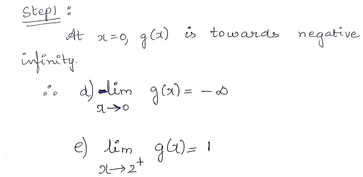
![### Graph Analysis and Limits
The image features a graph of the function \( g(x) \) plotted on a coordinate plane. The graph exhibits various behaviors such as oscillations, peaks, and asymptotes.
#### Given Limits:
- **(a)** \(\lim_{{x \to \infty}} g(x) = 2\) ✔️
- **(b)** \(\lim_{{x \to -\infty}} g(x) = -2\) ✔️
- **(c)** \(\lim_{{x \to 3}} g(x) = \text{infinity}\) ✔️
- **(d)** \(\lim_{{x \to 0}} g(x) =\)
- **(e)** \(\lim_{{x \to 2^{+}}} g(x) =\)
#### Asymptotes:
**(f)** The equations of the asymptotes. (Select all that apply.)
- [ ] \( x = -3 \)
- [ ] \( x = -2 \)
- [ ] \( x = 0 \)
- [ ] \( x = 2 \)
- [ ] \( x = 3 \)
### Graph Explanation:
The graph shows the function \( g(x) \) with various key characteristics:
1. **Horizontal Behavior:**
- As \( x \) approaches infinity, the function approaches a horizontal asymptote at \( y = 2 \).
- As \( x \) approaches negative infinity, the function approaches another horizontal asymptote at \( y = -2 \).
2. **Vertical Asymptote:**
- At \( x = 3 \), the graph shows a vertical asymptote as the limit approaches infinity.
3. **Unlabeled Points:**
- The graph suggests potential vertical asymptotes at the points to evaluate in section (d) and (e), such as \( x = 0 \) and \( x = 2^+ \), but these are not explicitly solved in the provided options.
This information can be used to interpret the behavior of the function \( g(x) \) as it approaches the specified points or extends toward infinity.](/v2/_next/image?url=https%3A%2F%2Fcontent.bartleby.com%2Fqna-images%2Fquestion%2F1e6ee9ac-917d-48ac-8e12-6329174ebdc0%2F3bf2effa-652d-4b71-b5b4-7daa63dfba34%2Fu9a2749.jpeg&w=3840&q=75)
Transcribed Image Text:### Graph Analysis and Limits
The image features a graph of the function \( g(x) \) plotted on a coordinate plane. The graph exhibits various behaviors such as oscillations, peaks, and asymptotes.
#### Given Limits:
- **(a)** \(\lim_{{x \to \infty}} g(x) = 2\) ✔️
- **(b)** \(\lim_{{x \to -\infty}} g(x) = -2\) ✔️
- **(c)** \(\lim_{{x \to 3}} g(x) = \text{infinity}\) ✔️
- **(d)** \(\lim_{{x \to 0}} g(x) =\)
- **(e)** \(\lim_{{x \to 2^{+}}} g(x) =\)
#### Asymptotes:
**(f)** The equations of the asymptotes. (Select all that apply.)
- [ ] \( x = -3 \)
- [ ] \( x = -2 \)
- [ ] \( x = 0 \)
- [ ] \( x = 2 \)
- [ ] \( x = 3 \)
### Graph Explanation:
The graph shows the function \( g(x) \) with various key characteristics:
1. **Horizontal Behavior:**
- As \( x \) approaches infinity, the function approaches a horizontal asymptote at \( y = 2 \).
- As \( x \) approaches negative infinity, the function approaches another horizontal asymptote at \( y = -2 \).
2. **Vertical Asymptote:**
- At \( x = 3 \), the graph shows a vertical asymptote as the limit approaches infinity.
3. **Unlabeled Points:**
- The graph suggests potential vertical asymptotes at the points to evaluate in section (d) and (e), such as \( x = 0 \) and \( x = 2^+ \), but these are not explicitly solved in the provided options.
This information can be used to interpret the behavior of the function \( g(x) \) as it approaches the specified points or extends toward infinity.
Expert Solution
Step 1

Step by step
Solved in 2 steps with 2 images

Recommended textbooks for you
Calculus: Early Transcendentals
Calculus
ISBN:
9781285741550
Author:
James Stewart
Publisher:
Cengage Learning

Thomas' Calculus (14th Edition)
Calculus
ISBN:
9780134438986
Author:
Joel R. Hass, Christopher E. Heil, Maurice D. Weir
Publisher:
PEARSON

Calculus: Early Transcendentals (3rd Edition)
Calculus
ISBN:
9780134763644
Author:
William L. Briggs, Lyle Cochran, Bernard Gillett, Eric Schulz
Publisher:
PEARSON
Calculus: Early Transcendentals
Calculus
ISBN:
9781285741550
Author:
James Stewart
Publisher:
Cengage Learning
Thomas' Calculus (14th Edition)
Calculus
ISBN:
9780134438986
Author:
Joel R. Hass, Christopher E. Heil, Maurice D. Weir
Publisher:
PEARSON
Calculus: Early Transcendentals (3rd Edition)
Calculus
ISBN:
9780134763644
Author:
William L. Briggs, Lyle Cochran, Bernard Gillett, Eric Schulz
Publisher:
PEARSON

Calculus: Early Transcendentals
Calculus
ISBN:
9781319050740
Author:
Jon Rogawski, Colin Adams, Robert Franzosa
Publisher:
W. H. Freeman


Calculus: Early Transcendental Functions
Calculus
ISBN:
9781337552516
Author:
Ron Larson, Bruce H. Edwards
Publisher:
Cengage Learning