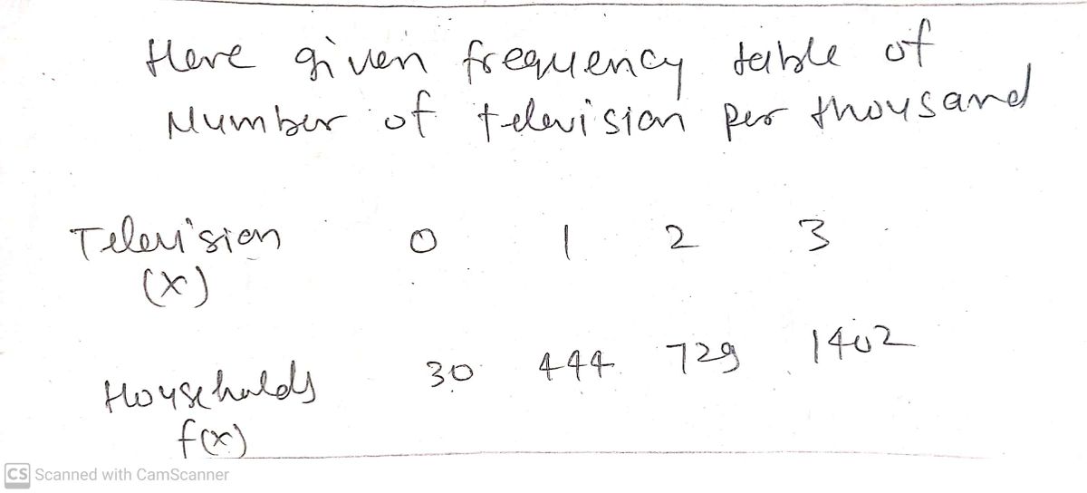
I am having a hard time trying to understand this topic. My TI-84 calculator has stopped working and I'm having to figure this out by hand. **Frequency Distribution in a Small Town**A frequency distribution is presented below for the number of televisions per household in a small town.| Televisions | Households ||-------------|------------|| 0 | 30 || 1 | 444 || 2 | 729 || 3 | 1402 |**Tasks:**(a) **Probability Table**- Probability for 2 televisions: 0.353- Probability for 3 televisions: 0.679- (Round probabilities to the nearest thousandth as needed.)(b) **Mean of the Probability Distribution**- Mean (μ) = 2.9 (Round to the nearest tenth as needed.)**Additional Calculations:**- **Variance (σ²) of the Probability Distribution:** - Calculation is required (Round to the nearest tenth as needed.)- **Standard Deviation (σ) of the Probability Distribution:** - Calculation is required (Round to the nearest tenth as needed.)This information can help to understand the distribution and average number of televisions per household, alongside variability within the surveyed households. ### Understanding Frequency and Probability DistributionsThe following data represents the number of televisions per household in a small town:| Televisions | Households ||-------------|------------|| 0 | 30 || 1 | 444 || 2 | 729 || 3 | 1402 |#### (a) Constructing a Probability DistributionUsing the frequency distribution, we can create a probability distribution as follows:| x | P(x) ||---|-------|| 0 | 0.012 || 1 | 0.170 || 2 | 0.353 || 3 | 0.679 |*(Note: Probabilities are rounded to the nearest thousandth.)*#### (b) Calculating the Mean of the Probability DistributionTo find the mean (μ) of the probability distribution:\[ \mu = 2.9 \]*(Rounded to the nearest tenth as needed.)*#### Calculating the Variance of the Probability DistributionThe variance (σ²) is also calculated but is not visible in this image. However, it typically follows the formula for variance of a probability distribution:\[ \sigma^2 = \sum [x^2 \cdot P(x)] - \mu^2 \]### ExplanationThe data shows that most households have 3 televisions, as indicated by the largest number in the frequency table (1402 households). The probability distribution provides a view of the likelihood of each possible outcome, with the highest probability (0.679) being for 3 televisions per household. The mean gives an average of about 2.9 televisions per household.

Answered: Image /qna-images/answer/22bfb8b8-edcc-4671-af89-667a2501c2dc.jpg

Answered: A frequency distribution is shown…

A frequency distribution is shown below. Complete parts (a) through (d). The number of televisions per household in a small town Televisions 0 1 2 3 Households 30 444 729 1402 2 0.353

A First Course in Probability (10th Edition)

10th Edition

ISBN:9780134753119

Author:Sheldon Ross

Publisher:Sheldon Ross

Chapter1: Combinatorial Analysis

Section: Chapter Questions

Problem 1.1P: a. How many different 7-place license plates are possible if the first 2 places are for letters and...

See similar textbooks

Similar questions

While working on the multiplication problem 38 x 25, Maria says this: “Four times 25 is 100, so 40 times 25 is 1000. Now take away 2, so the answer is 998.” Is Maria’s method correct or not? If it is correct, write equations that incorporate Maria’s work and that show why it’s correct. If Maria’s reasoning is not correct, explain why. Work with portions that are right to correct Maria’s work, and write a string of equations that corresponds to your corrected method for calculating 38 x 25. In either case, write your equations in the following form:
I don't understand how part is broken down
USA. Benjamin Banneker (1731-1806) is one of the great American heroes of all time. The son and grandson of Africans captured and enslaved, he was fortunate to have been born free. He inherited the family farm where he worked hard all of his life. As a child he had a few months of schooling. Everything else he had to do on his own. He loved mathematics and science but did not get a chance to learn astronomy until he was in his fifties. Then he performed a near miracle, learning it all in less than a year. In his hand-written journal, he recorded two right triangle examples that interested him. You can solve them here and remember the great man who enjoyed geometry. On the page in his journal next to the August 1775 astronomy calculations, Banneker wrote, in the style of that time: Suppose a ladder 60 feet long be placed in a Street so as to reach a window on the one Side 37 feet high, and without moving it at bottom, will reach another window on the other side of teh Street which is 23…
Please Explain Clearly because I'm having a hard time understanding this material?
I need some explanation on these 3 problems.
Can you help me please! How did the mathematical concepts that developed during Arabic period have an impact on modern mathematics? Discuss the cultural and historical setting during Arabic period.
Identify two problems with the following question. Explain how you would rewrite it so that it is more appropriate.given that youth crime is on the rise in urban areas, what should be the top enforcement priority for our local police force? which one is correct answer? 1.youth crime 2.car theft 3.illegal drug use 4.violent crime
Dear tutor, please help me solve this calculas question
doesn't make sense. can you please explain a bit better?
Direction: Analyze the given problem and show your complete and detailed solution using multiplication priniciple. A special plate number is made of three letters in the English Alphabet followed by two-digit numbers. How many plate numbers are possible if (a) the digits and letters can be repeated in the same plate number (b) the letters and digits cannot be repeated in the same plate number.
Can you help me find answer for this question?
I'm confused on how to do the second part of the problem still.