4.13 The linear regression model is y = B₁ + B₂x + e. Let y be the sample mean of the y-values and the average of the x-values. Create variables y = y-y and x = x-x. Let y = ax + e. a. Show, algebraically, that the least squares estimator of a is identical to the least square estimator of ß₂. [Hint: See Exercise 2.4.] b. Show, algebraically, that the least squares residuals from ỹ = ax + e are the same as the least squares residuals from the original linear model y =B₁ + B₂x + e.
4.13 The linear regression model is y = B₁ + B₂x + e. Let y be the sample mean of the y-values and the average of the x-values. Create variables y = y-y and x = x-x. Let y = ax + e. a. Show, algebraically, that the least squares estimator of a is identical to the least square estimator of ß₂. [Hint: See Exercise 2.4.] b. Show, algebraically, that the least squares residuals from ỹ = ax + e are the same as the least squares residuals from the original linear model y =B₁ + B₂x + e.

MATLAB: An Introduction with Applications
6th Edition
ISBN:9781119256830
Author:Amos Gilat
Publisher:Amos Gilat
Chapter1: Starting With Matlab
Section: Chapter Questions
Problem 1P

Related questions
Question
100%
Please answer 4.13
![to the budget share relation?
f. The least squares estimates of In(FOOD) = a₁ + a₂ln(TOTEXP) + e are as follows:
ô = 0.2729
In(FOOD) = 0.732 +0.608 In(TOTEXP) R² = 0.4019
(6.58) (24.91)
Interpret the estimated coefficient of In(TOTEXP). Calculate the elasticity in this model at the 5th
percentile and the 75th percentile of total expenditure. Is this a constant elasticity function?
g. The residuals from the log-log model in (e) show skewness = -0.887 and kurtosis = 5.023. Carry
out the Jarque-Bera test at the 5% level of significance.
h. In addition to the information in the previous parts, we multiply the fitted value in part (b) by
TOTEXP to obtain a prediction for expenditure on food. The correlation between this value and
actual food expenditure is 0.641. Using the model in part (e) we obtain exp [In(FOOD)]. The cor-
relation between this value and actual expenditure on food is 0.640. What if any information is
provided by these correlations? Which model would you select for reporting, if you had to choose
only one? Explain your choice.
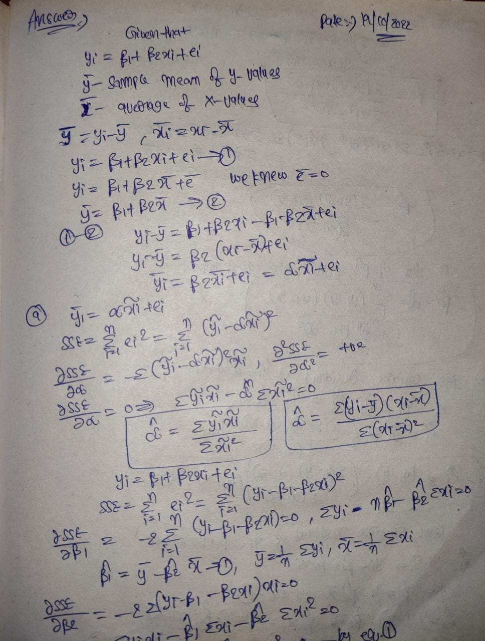
4.13 The linear regression model is y = B₁ + B₂x+e. Let y be the sample mean of the y-values and the
average of the x-values. Create variables y = y-y and x = x-x. Letỹ = ax + e.
a. Show, algebraically, that the least squares estimator of a is identical to the least square estimator
of B₂. [Hint: See Exercise 2.4.]
b. Show, algebraically, that the least squares residuals from y = ax + e are the same as the least
squares residuals from the original linear model y = B₁ + B₂x + e.
4.14 Using data on 5766 primary school children, we estimate two models relating their performance on a
math test (MATHSCORE) to their teacher's years of experience (TCHEXPER).
Linear relationship
MATHSCORE=478.15 +0.81TCHEXPER R2 = 0.0095 = 47.51
(1.19) (0.11)
(se)
Linear-log relationship
MATHSCORE= 474.25 +5.63 In(TCHEXPER) R2 = 0.0081 = 47.57
(se)
(1.84) (0.84)
a. Using the linear fitted relationship, how many years of additional teaching experience is required
to increase the expected math score by 10 points? Explain your calculation.
b. Does the linear fitted relationship imply that at some point there are diminishing returns to addi-
tional years of teaching experience? Explain.
c. Using the fitted linear-log model, is the graph of MA
a constant rate, at an increasing rate, or at a decrea
the fitted linear relationship?
d. Using the linear-log fitted relationship,
years of extra teaching experience is r
Explain your calculation.
e. 252 of the teachers had no teaching exp
two models?
f. These models have such a low R2 th
expected math score and years of teach
4.15 Consider a log-reciprocal model that relat
cal of the explanatory variable, In(y) = P₁
Exercise 4.17].
a. For what values of y is this model define
b. Write the model in exponential form as
tionship is dy/dx = exp[B, + (B₂/x)]>
X
ag that r>0
er
gai
b
ic
XA
t
7
PER increasing at
this compare to
ce, how many
by 10 s?](/v2/_next/image?url=https%3A%2F%2Fcontent.bartleby.com%2Fqna-images%2Fquestion%2F6b1ec9e1-71c5-41a7-88e5-1ec0b0e62692%2F68dd922d-3b03-4bb6-9bca-c71a183594fa%2Fw39kwio_processed.jpeg&w=3840&q=75)
Transcribed Image Text:to the budget share relation?
f. The least squares estimates of In(FOOD) = a₁ + a₂ln(TOTEXP) + e are as follows:
ô = 0.2729
In(FOOD) = 0.732 +0.608 In(TOTEXP) R² = 0.4019
(6.58) (24.91)
Interpret the estimated coefficient of In(TOTEXP). Calculate the elasticity in this model at the 5th
percentile and the 75th percentile of total expenditure. Is this a constant elasticity function?
g. The residuals from the log-log model in (e) show skewness = -0.887 and kurtosis = 5.023. Carry
out the Jarque-Bera test at the 5% level of significance.
h. In addition to the information in the previous parts, we multiply the fitted value in part (b) by
TOTEXP to obtain a prediction for expenditure on food. The correlation between this value and
actual food expenditure is 0.641. Using the model in part (e) we obtain exp [In(FOOD)]. The cor-
relation between this value and actual expenditure on food is 0.640. What if any information is
provided by these correlations? Which model would you select for reporting, if you had to choose
only one? Explain your choice.
4.13 The linear regression model is y = B₁ + B₂x+e. Let y be the sample mean of the y-values and the
average of the x-values. Create variables y = y-y and x = x-x. Letỹ = ax + e.
a. Show, algebraically, that the least squares estimator of a is identical to the least square estimator
of B₂. [Hint: See Exercise 2.4.]
b. Show, algebraically, that the least squares residuals from y = ax + e are the same as the least
squares residuals from the original linear model y = B₁ + B₂x + e.
4.14 Using data on 5766 primary school children, we estimate two models relating their performance on a
math test (MATHSCORE) to their teacher's years of experience (TCHEXPER).
Linear relationship
MATHSCORE=478.15 +0.81TCHEXPER R2 = 0.0095 = 47.51
(1.19) (0.11)
(se)
Linear-log relationship
MATHSCORE= 474.25 +5.63 In(TCHEXPER) R2 = 0.0081 = 47.57
(se)
(1.84) (0.84)
a. Using the linear fitted relationship, how many years of additional teaching experience is required
to increase the expected math score by 10 points? Explain your calculation.
b. Does the linear fitted relationship imply that at some point there are diminishing returns to addi-
tional years of teaching experience? Explain.
c. Using the fitted linear-log model, is the graph of MA
a constant rate, at an increasing rate, or at a decrea
the fitted linear relationship?
d. Using the linear-log fitted relationship,
years of extra teaching experience is r
Explain your calculation.
e. 252 of the teachers had no teaching exp
two models?
f. These models have such a low R2 th
expected math score and years of teach
4.15 Consider a log-reciprocal model that relat
cal of the explanatory variable, In(y) = P₁
Exercise 4.17].
a. For what values of y is this model define
b. Write the model in exponential form as
tionship is dy/dx = exp[B, + (B₂/x)]>
X
ag that r>0
er
gai
b
ic
XA
t
7
PER increasing at
this compare to
ce, how many
by 10 s?
Expert Solution
Step 1

Step by step
Solved in 4 steps with 4 images

Recommended textbooks for you
MATLAB: An Introduction with Applications
Statistics
ISBN:
9781119256830
Author:
Amos Gilat
Publisher:
John Wiley & Sons Inc

Probability and Statistics for Engineering and th…
Statistics
ISBN:
9781305251809
Author:
Jay L. Devore
Publisher:
Cengage Learning

Statistics for The Behavioral Sciences (MindTap C…
Statistics
ISBN:
9781305504912
Author:
Frederick J Gravetter, Larry B. Wallnau
Publisher:
Cengage Learning
MATLAB: An Introduction with Applications
Statistics
ISBN:
9781119256830
Author:
Amos Gilat
Publisher:
John Wiley & Sons Inc
Probability and Statistics for Engineering and th…
Statistics
ISBN:
9781305251809
Author:
Jay L. Devore
Publisher:
Cengage Learning
Statistics for The Behavioral Sciences (MindTap C…
Statistics
ISBN:
9781305504912
Author:
Frederick J Gravetter, Larry B. Wallnau
Publisher:
Cengage Learning

Elementary Statistics: Picturing the World (7th E…
Statistics
ISBN:
9780134683416
Author:
Ron Larson, Betsy Farber
Publisher:
PEARSON

The Basic Practice of Statistics
Statistics
ISBN:
9781319042578
Author:
David S. Moore, William I. Notz, Michael A. Fligner
Publisher:
W. H. Freeman

Introduction to the Practice of Statistics
Statistics
ISBN:
9781319013387
Author:
David S. Moore, George P. McCabe, Bruce A. Craig
Publisher:
W. H. Freeman