23Help
Contingency Table
A contingency table can be defined as the visual representation of the relationship between two or more categorical variables that can be evaluated and registered. It is a categorical version of the scatterplot, which is used to investigate the linear relationship between two variables. A contingency table is indeed a type of frequency distribution table that displays two variables at the same time.
Binomial Distribution
Binomial is an algebraic expression of the sum or the difference of two terms. Before knowing about binomial distribution, we must know about the binomial theorem.
23Help


Hello there! there are more than three subparts in the question. According to our policies we cannot answer more than three sub parts in one question. So please find the solution for a,b,c parts of the question. If you have doubts in remaining part of the question kindly make a new request, mentioning the part in which you need help.
Given data
H0:µ = 49
H1:µ ≠ 49
a)
Points on sampling distribution of the sample mean:
- If the true population distribution of a random variable, say, x, is normal with parameters, mean μ and standard deviation σ, then, whatever be the size (n) of the sample taken from the population, the distribution of the sample mean is also normal, with parameters, mean μ and standard deviation σ/√n.
- Even if the true population distribution of a random variable, say, x, is not normal and has population mean μ, standard deviation σ, then, for a large size (n ≥ 30) of a sample taken from the population, the distribution of the sample mean is approximately normal, with parameters, mean μ and standard deviation σ/√n (by Central Limit Theorem).
- If the true population distribution of a random variable, say, x, is not normal and has population mean μ, standard deviation σ, then, for a small size (n < 30) of a sample taken from the population, the distribution of the sample mean cannot be said to be approximately normal.
So, from the above, option B is correct.
No – Since the sample size is at least 30, the underlying population does not need to be normally distributed.
b)
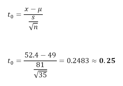
x̅ = 52.4, s = 81
Test statistic is given by

Step by step
Solved in 3 steps with 1 images


