Chapter 4.3, Problem 1SP

Lord Kelvin and the Age of Earth

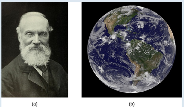Figure 4.25 (a) William Thomson (Lord Kelvin). 1824-1907, was a British physicist and electrical engineer. (b) Kelvin used the heat diffusion equation to estimate the age of Earth (credit: modification of work by NASA).

During the late 1800s, the scientists of the new field of geology were coming to the conclusion the Earth must be “millions and millions” of years old. At about the same time. Charles Darwin had published his treatise on evolution.

Darwin’s view was that evolution needed many millions of years to take place, and he made a bold claim that the Weald chalk fields, where important fossils were found, were the result of 300 million years of erosion.

At that time, eminent physicist William Thomson (lord Kelvin) used an important partial differential equation, known as the heat diffusion equation, to estimate the age of Earth by determining how long it would take Earth to cool from molten rock to what we had at tha time. His conclusion was a range of 20 to 4(X) million years, but most likely about 5() million years. For many decades, the proclamations of this irrefutable icon of science did not sit well with geologists or with Darwin.

tJR ead Kelvin’s paper (http:Iiwww.openstaxcollege.orgIlI2O KelEarthAge) on estimating the age of the Earth.

Kelvin made reasonable assumptions based on what was known in his time, but he also made several assumptions that turned out to be wrong. One incorrect assumption was that Earth is solid and that the cooling was therefore via conduction only, hence justifying the use of the diffusion equation. But the most serious error was a forgivable one—omission of the fact that Earth contains radioactive elements that continually supply heat beneath Earth’s mantle. The discoveiy of radioactivity came near the end of Kelvin’s life and he acknowledged that his calculation would have to be modified.

Kelvin used the simple one-dimensional model applied only to Earth’s outer shell, and derived the age from gsaphs and the roughly known temperature gs-adietn near Earth’s surface. Let’s take a look at a more appropriate version of the diffusion equation in radial coordinates, which has the form

   $\frac{\partial T}{\partial t}=K\left[\frac{{\partial }^{2}T}{{\partial }^{2}r}+\frac{2}{r}\frac{\partial T}{\partial r}\right]$

(4.23)

Here, T(r.t) is temperature as a function of r (measured from the center of Earth) and time i. K is the heat conductivity—for molten rock, in this case. ibe standard method of solving such a partial differential equation is by separation of variables, where we express the solution as the product of functions containing each variable separately. In this case, we would write the temperature as

$T\left(r,t\right)=R\left(r\right)f\left(t\right).$