Statistical Reasoning for Everyday Life (5th Edition)
5th Edition
ISBN: 9780134494043
Author: Jeff Bennett, William L. Briggs, Mario F. Triola
Publisher: PEARSON
expand_more
expand_more
format_list_bulleted
Concept explainers
Videos
Textbook Question
Chapter 3.2, Problem 17E
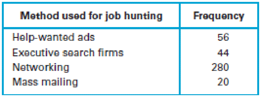
Job Hunting. A survey was conducted to determine how employees found their jobs. The table below lists the successful methods identified by 400 randomly selected employees. The data are based on results from the National Center for Career Strategies. Construct a Pareto chart that displays the given data. Based on these results, what appears to be the best method for someone seeking employment?
Expert Solution & Answer
Want to see the full answer?
Check out a sample textbook solution
Students have asked these similar questions
A major company in the Montreal area, offering a range of engineering services from project preparation to construction execution, and industrial project management, wants to ensure that the individuals who are responsible for project cost estimation and bid preparation demonstrate a certain uniformity in their estimates. The head of civil engineering and municipal services decided to structure an experimental plan to detect if there could be significant differences in project evaluation.
Seven projects were selected, each of which had to be evaluated by each of the two estimators, with the order of the projects submitted being random. The obtained estimates are presented in the table below.
a) Complete the table above by calculating: i. The differences (A-B) ii. The sum of the differences iii. The mean of the differences iv. The standard deviation of the differences
b) What is the value of the t-statistic?
c) What is the critical t-value for this test at a significance level of 1%?…
Compute the relative risk of falling for the two groups (did not stop walking vs. did stop). State/interpret your result verbally.
Microsoft Excel include formulas
Chapter 3 Solutions
Statistical Reasoning for Everyday Life (5th Edition)
Ch. 3.1 - Frequency Table. What is a frequency table? How...Ch. 3.1 - Relative Frequency. What do we mean by relative...Ch. 3.1 - Cumulative Frequency. What do we mean by...Ch. 3.1 - Binning. What is the purpose of binning? Give an...Ch. 3.1 - Does It Make Sense? For Exercises 58, determine...Ch. 3.1 - Does It Make Sense? For Exercises 58, determine...Ch. 3.1 - Does It Make Sense? For Exercises 58, determine...Ch. 3.1 - Does It Make Sense? For Exercises 58, determine...Ch. 3.1 - Pulse Rates of Females. In Exercises 912, refer to...Ch. 3.1 - Pulse Rates of Females. In Exercises 912, refer to...
Ch. 3.1 - Pulse Rates of Females. In Exercises 912, refer to...Ch. 3.1 - Pulse Rates of Females. In Exercises 912, refer to...Ch. 3.1 - Birth Days. Births at a hospital in New York State...Ch. 3.1 - Clinical Trial. As part of a clinical trial, the...Ch. 3.1 - Train Derailments. An analysis of 50 train...Ch. 3.1 - Analysis of Last Digits. Weights of respondents...Ch. 3.1 - Academy Award-Winning Male Actors. The following...Ch. 3.1 - Body Temperatures. The following data show the...Ch. 3.1 - Loaded Die. An experiment was conducted in which a...Ch. 3.1 - Interpreting Family Data. Consider the following...Ch. 3.1 - Computer Keyboards. The traditional keyboard...Ch. 3.1 - Double Binning. The students in a statistics class...Ch. 3.2 - Distribution Graph. What is a distribution of...Ch. 3.2 - Qualitative Data. Which types of graph described...Ch. 3.2 - Yearly Data. Which type of graph described in this...Ch. 3.2 - Histogram and Stemplot. Assume that a data set is...Ch. 3.2 - Prob. 5ECh. 3.2 - Does It Make Sense? For Exercises 58, determine...Ch. 3.2 - Does It Make Sense? For Exercises 58, determine...Ch. 3.2 - Does It Make Sense? For Exercises 58, determine...Ch. 3.2 - Histogram. Children living near a smelter in Texas...Ch. 3.2 - Understanding Data. Suppose you have a list of...Ch. 3.2 - Most Appropriate Display. Exercises 1114 describe...Ch. 3.2 - Most Appropriate Display. Exercises 1114 describe...Ch. 3.2 - Most Appropriate Display. Exercises 1114 describe...Ch. 3.2 - Most Appropriate Display. Exercises 1114 describe...Ch. 3.2 - Academy Award-Winning Male Actors. Exercise 17 in...Ch. 3.2 - Body Temperatures. Exercise 18 in Section 3.1...Ch. 3.2 - Job Hunting. A survey was conducted to determine...Ch. 3.2 - Job Hunting. Refer to the data given in Exercise...Ch. 3.2 - Prob. 19ECh. 3.2 - Job Application Mistakes Construct a Pareto chart...Ch. 3.2 - Dotplot. Refer to the QWERTY data in Exercise 21...Ch. 3.2 - Dotplot. Refer to the Dvorak data in Exercise 21...Ch. 3.2 - Stemplot. Construct a stemplot of these test...Ch. 3.2 - Stemplot. Listed below are the lengths (in...Ch. 3.2 - DJIA. Listed below (in order by row) are annual...Ch. 3.2 - Home Runs. Listed below (in order by row) are the...Ch. 3.3 - Multiple Data. Briefly describe how each of the...Ch. 3.3 - Prob. 2ECh. 3.3 - Prob. 3ECh. 3.3 - Prob. 4ECh. 3.3 - Does It Make Sense? For Exercises 58, determine...Ch. 3.3 - Does It Make Sense? For Exercises 58, determine...Ch. 3.3 - Does It Make Sense? For Exercises 58, determine...Ch. 3.3 - Does It Make Sense? For Exercises 58, determine...Ch. 3.3 - Public and Private Colleges. The stack plot in...Ch. 3.3 - Home Prices by Region. The graph in Figure 3.21...Ch. 3.3 - Gender and Salary. Consider the display in Figure...Ch. 3.3 - Marriage and Divorce Rates. The graph in Figure...Ch. 3.3 - Prob. 13ECh. 3.3 - College Degrees. The stack plot in Figure 3.25...Ch. 3.3 - Contour Map. For Exercises 17 and 18, refer to the...Ch. 3.3 - Prob. 18ECh. 3.3 - Prob. 19ECh. 3.3 - Prob. 20ECh. 3.3 - Infographic. For Exercises 21 and 22, refer to...Ch. 3.3 - Infographic. For Exercises 21 and 22, refer to...Ch. 3.3 - Creating Graphics. Exercises 2326 give tables of...Ch. 3.3 - Creating Graphics. Exercises 2326 give tables of...Ch. 3.3 - Firearms Fatalities. The following table...Ch. 3.3 - Prob. 26ECh. 3.4 - Perceptual Distortion. Use a ruler to measure the...Ch. 3.4 - Prob. 2ECh. 3.4 - Prob. 3ECh. 3.4 - Prob. 4ECh. 3.4 - Does It Make Sense? For Exercises 58, determine...Ch. 3.4 - Does It Make Sense? For Exercises 58, determine...Ch. 3.4 - Does It Make Sense? For Exercises 58, determine...Ch. 3.4 - Does It Make Sense? For Exercises 58, determine...Ch. 3.4 - Exaggerating a Difference. Weekly instruction time...Ch. 3.4 - Graph of Sounds. In a survey conducted by Kelton...Ch. 3.4 - Graph Dimensions. A newspaper used images of...Ch. 3.4 - Prob. 12ECh. 3.4 - Prob. 13ECh. 3.4 - DJIA. Figure 3.36 on the next page depicts the...Ch. 3.4 - Prob. 15ECh. 3.4 - Prob. 16ECh. 3.4 - Prob. 17ECh. 3.4 - Moores Law. In 1965, Intel cofounder Gordon Moore...Ch. 3.4 - Prob. 19ECh. 3.4 - Prob. 20ECh. 3.4 - Constant Dollars. The graph in Figure 3.41 shows...Ch. 3.4 - Prob. 22ECh. 3 - Listed below are measured weights (in pounds) of...Ch. 3 - Listed below are measured weights (in pounds) of...Ch. 3 - Listed below are measured weights (in pounds) of...Ch. 3 - Pie Chart for Sports Equipment. USA Today reported...Ch. 3 - Pareto Chart for Sports Equipment. Construct a...Ch. 3 - Bar Chart. Figure 3.43 shows the numbers of U.S....Ch. 3 - As a quality control manager at Ford Motor...Ch. 3 - As a quality control manager at Ford, you monitor...Ch. 3 - A stemplot is created with the braking distances...Ch. 3 - A dotplot of braking distances (in feet) of cars...Ch. 3 - The first category in a frequency table is 90100,...Ch. 3 - The first category in a relative frequency table...Ch. 3 - The third category in a frequency table has a...Ch. 3 - Prob. 8CQCh. 3 - When constructing a graph of the same categorical...Ch. 3 - Body Temperatures Listed below are body...Ch. 3 - Why are pictographs generally poor for depicting...Ch. 3 - Note that this graph plots six variables: two...Ch. 3 - Prob. 2.2FCh. 3 - Prob. 2.3F
Knowledge Booster


Learn more about
Need a deep-dive on the concept behind this application? Look no further. Learn more about this topic, statistics and related others by exploring similar questions and additional content below.Similar questions
- Question 1 The data shown in Table 1 are and R values for 24 samples of size n = 5 taken from a process producing bearings. The measurements are made on the inside diameter of the bearing, with only the last three decimals recorded (i.e., 34.5 should be 0.50345). Table 1: Bearing Diameter Data Sample Number I R Sample Number I R 1 34.5 3 13 35.4 8 2 34.2 4 14 34.0 6 3 31.6 4 15 37.1 5 4 31.5 4 16 34.9 7 5 35.0 5 17 33.5 4 6 34.1 6 18 31.7 3 7 32.6 4 19 34.0 8 8 33.8 3 20 35.1 9 34.8 7 21 33.7 2 10 33.6 8 22 32.8 1 11 31.9 3 23 33.5 3 12 38.6 9 24 34.2 2 (a) Set up and R charts on this process. Does the process seem to be in statistical control? If necessary, revise the trial control limits. [15 pts] (b) If specifications on this diameter are 0.5030±0.0010, find the percentage of nonconforming bearings pro- duced by this process. Assume that diameter is normally distributed. [10 pts] 1arrow_forward4. (5 pts) Conduct a chi-square contingency test (test of independence) to assess whether there is an association between the behavior of the elderly person (did not stop to talk, did stop to talk) and their likelihood of falling. Below, please state your null and alternative hypotheses, calculate your expected values and write them in the table, compute the test statistic, test the null by comparing your test statistic to the critical value in Table A (p. 713-714) of your textbook and/or estimating the P-value, and provide your conclusions in written form. Make sure to show your work. Did not stop walking to talk Stopped walking to talk Suffered a fall 12 11 Totals 23 Did not suffer a fall | 2 Totals 35 37 14 46 60 Tarrow_forwardQuestion 2 Parts manufactured by an injection molding process are subjected to a compressive strength test. Twenty samples of five parts each are collected, and the compressive strengths (in psi) are shown in Table 2. Table 2: Strength Data for Question 2 Sample Number x1 x2 23 x4 x5 R 1 83.0 2 88.6 78.3 78.8 3 85.7 75.8 84.3 81.2 78.7 75.7 77.0 71.0 84.2 81.0 79.1 7.3 80.2 17.6 75.2 80.4 10.4 4 80.8 74.4 82.5 74.1 75.7 77.5 8.4 5 83.4 78.4 82.6 78.2 78.9 80.3 5.2 File Preview 6 75.3 79.9 87.3 89.7 81.8 82.8 14.5 7 74.5 78.0 80.8 73.4 79.7 77.3 7.4 8 79.2 84.4 81.5 86.0 74.5 81.1 11.4 9 80.5 86.2 76.2 64.1 80.2 81.4 9.9 10 75.7 75.2 71.1 82.1 74.3 75.7 10.9 11 80.0 81.5 78.4 73.8 78.1 78.4 7.7 12 80.6 81.8 79.3 73.8 81.7 79.4 8.0 13 82.7 81.3 79.1 82.0 79.5 80.9 3.6 14 79.2 74.9 78.6 77.7 75.3 77.1 4.3 15 85.5 82.1 82.8 73.4 71.7 79.1 13.8 16 78.8 79.6 80.2 79.1 80.8 79.7 2.0 17 82.1 78.2 18 84.5 76.9 75.5 83.5 81.2 19 79.0 77.8 20 84.5 73.1 78.2 82.1 79.2 81.1 7.6 81.2 84.4 81.6 80.8…arrow_forward
- Name: Lab Time: Quiz 7 & 8 (Take Home) - due Wednesday, Feb. 26 Contingency Analysis (Ch. 9) In lab 5, part 3, you will create a mosaic plot and conducted a chi-square contingency test to evaluate whether elderly patients who did not stop walking to talk (vs. those who did stop) were more likely to suffer a fall in the next six months. I have tabulated the data below. Answer the questions below. Please show your calculations on this or a separate sheet. Did not stop walking to talk Stopped walking to talk Totals Suffered a fall Did not suffer a fall Totals 12 11 23 2 35 37 14 14 46 60 Quiz 7: 1. (2 pts) Compute the odds of falling for each group. Compute the odds ratio for those who did not stop walking vs. those who did stop walking. Interpret your result verbally.arrow_forwardSolve please and thank you!arrow_forward7. In a 2011 article, M. Radelet and G. Pierce reported a logistic prediction equation for the death penalty verdicts in North Carolina. Let Y denote whether a subject convicted of murder received the death penalty (1=yes), for the defendant's race h (h1, black; h = 2, white), victim's race i (i = 1, black; i = 2, white), and number of additional factors j (j = 0, 1, 2). For the model logit[P(Y = 1)] = a + ß₁₂ + By + B²², they reported = -5.26, D â BD = 0, BD = 0.17, BY = 0, BY = 0.91, B = 0, B = 2.02, B = 3.98. (a) Estimate the probability of receiving the death penalty for the group most likely to receive it. [4 pts] (b) If, instead, parameters used constraints 3D = BY = 35 = 0, report the esti- mates. [3 pts] h (c) If, instead, parameters used constraints Σ₁ = Σ₁ BY = Σ; B = 0, report the estimates. [3 pts] Hint the probabilities, odds and odds ratios do not change with constraints.arrow_forward
- Solve please and thank you!arrow_forwardSolve please and thank you!arrow_forwardQuestion 1:We want to evaluate the impact on the monetary economy for a company of two types of strategy (competitive strategy, cooperative strategy) adopted by buyers.Competitive strategy: strategy characterized by firm behavior aimed at obtaining concessions from the buyer.Cooperative strategy: a strategy based on a problem-solving negotiating attitude, with a high level of trust and cooperation.A random sample of 17 buyers took part in a negotiation experiment in which 9 buyers adopted the competitive strategy, and the other 8 the cooperative strategy. The savings obtained for each group of buyers are presented in the pdf that i sent: For this problem, we assume that the samples are random and come from two normal populations of unknown but equal variances.According to the theory, the average saving of buyers adopting a competitive strategy will be lower than that of buyers adopting a cooperative strategy.a) Specify the population identifications and the hypotheses H0 and H1…arrow_forward
- You assume that the annual incomes for certain workers are normal with a mean of $28,500 and a standard deviation of $2,400. What’s the chance that a randomly selected employee makes more than $30,000?What’s the chance that 36 randomly selected employees make more than $30,000, on average?arrow_forwardWhat’s the chance that a fair coin comes up heads more than 60 times when you toss it 100 times?arrow_forwardSuppose that you have a normal population of quiz scores with mean 40 and standard deviation 10. Select a random sample of 40. What’s the chance that the mean of the quiz scores won’t exceed 45?Select one individual from the population. What’s the chance that his/her quiz score won’t exceed 45?arrow_forward
arrow_back_ios
SEE MORE QUESTIONS
arrow_forward_ios
Recommended textbooks for you
 College Algebra (MindTap Course List)AlgebraISBN:9781305652231Author:R. David Gustafson, Jeff HughesPublisher:Cengage Learning
 Holt Mcdougal Larson Pre-algebra: Student Edition...AlgebraISBN:9780547587776Author:HOLT MCDOUGALPublisher:HOLT MCDOUGAL
 Glencoe Algebra 1, Student Edition, 9780079039897...AlgebraISBN:9780079039897Author:CarterPublisher:McGraw Hill
 Big Ideas Math A Bridge To Success Algebra 1: Stu...AlgebraISBN:9781680331141Author:HOUGHTON MIFFLIN HARCOURTPublisher:Houghton Mifflin Harcourt
College Algebra (MindTap Course List)
Algebra
ISBN:9781305652231
Author:R. David Gustafson, Jeff Hughes
Publisher:Cengage Learning
Holt Mcdougal Larson Pre-algebra: Student Edition...
Algebra
ISBN:9780547587776
Author:HOLT MCDOUGAL
Publisher:HOLT MCDOUGAL
Glencoe Algebra 1, Student Edition, 9780079039897...
Algebra
ISBN:9780079039897
Author:Carter
Publisher:McGraw Hill
Big Ideas Math A Bridge To Success Algebra 1: Stu...
Algebra
ISBN:9781680331141
Author:HOUGHTON MIFFLIN HARCOURT
Publisher:Houghton Mifflin Harcourt
Probability & Statistics (28 of 62) Basic Definitions and Symbols Summarized; Author: Michel van Biezen;https://www.youtube.com/watch?v=21V9WBJLAL8;License: Standard YouTube License, CC-BY
Introduction to Probability, Basic Overview - Sample Space, & Tree Diagrams; Author: The Organic Chemistry Tutor;https://www.youtube.com/watch?v=SkidyDQuupA;License: Standard YouTube License, CC-BY