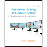
Spreadsheet Modeling & Decision Analysis: A Practical Introduction To Business Analytics, Loose-leaf Version
8th Edition
ISBN: 9781337274852
Author: Ragsdale, Cliff
Publisher: South-Western College Pub
expand_more
expand_more
format_list_bulleted
Concept explainers
Question
error_outline
This textbook solution is under construction.
Students have asked these similar questions
How would you monitor the strategy process to ensure that your strategic initiative succeeds? What should be monitored and why? Which Key Performance Indicators (KPIs) needed to be measured and monitored?
Compare and contrast descriptive statistics and inferential statistics. Explain the relationship of population, sampling frame, sampling design, and generalization.
The research methods used to collect data are Qualitative and Quantitative. If True, discuss. If False, discuss.
Knowledge Booster
Learn more about
Need a deep-dive on the concept behind this application? Look no further. Learn more about this topic, management and related others by exploring similar questions and additional content below.Similar questions
- Is it important to define the research problem before we collect the data?arrow_forwardContext: I'm a Business Management major in my senior year at University Question: What do you think is your strongest ability and how did you end up being good at it?arrow_forwardI'm a Business Management major in my senior year at University Question: What would you and others say are five of your personality pluses? And Why?arrow_forward
- I'm a Business Management major in my senior year at University Question: What new skills have you learned in the last year? And why were they worth learning?arrow_forwardof the various structures in place today, what do you see as the most beneficial to a technology-laden, forward-thinking organization, and why?arrow_forwardSarah Anderson, the Marketing Manager at Exeter Township's Cultural Center, is conducting research on the attendance history for cultural events in the area over the past ten years. The following data has been collected on the number of attendees who registered for events at the cultural center. Year Number of Attendees 1 700 2 248 3 633 4 458 5 1410 6 1588 7 1629 8 1301 9 1455 10 1989 You have been hired as a consultant to assist in implementing a forecasting system that utilizes various forecasting techniques to predict attendance for Year 11. a) Calculate the Three-Period Simple Moving Average b) Calculate the Three-Period Weighted Moving Average (weights: 50%, 30%, and 20%; use 50% for the most recent period, 30% for the next most recent, and 20% for the oldest) c) Apply Exponential Smoothing with the smoothing constant alpha = 0.2. d) Perform a Simple Linear Regression analysis and provide the adjusted…arrow_forward
- What tend to be the strengths and weaknesses of a group project in university? Describe.arrow_forwardCapsim Team PowerPoint Presentations - Slide Title: Final Results What were your Final Results with Broad Differentiation, R&D, Marketing, Awareness, and Accessibility strategies on your Capsim simulation?arrow_forwardCapsim Team PowerPoint Presentations - Slide Title: Strategy Overview Make bullet points about your achievements with Broad Differentiation, R&D, Marketing, Awareness, and Accessibility strategies on Capsim.arrow_forward
- Capsim Team PowerPoint Presentations - Slide Title: Strengths and Weaknesses of Your Team Describe the strengths and weaknesses of your team through your Capsim simulation.arrow_forwardCapsim Team PowerPoint Presentations - Slide Title: Major Decision PointWhat were your major decision points with Broad Differentiation, R&D, Marketing, Awareness, and Accessibility strategies on Capsim?arrow_forwardFor PurrTech’s expansion into Germany, I’ve decided to use a polycentric staffing approach—meaning we’ll hire German professionals to run our operations there. I believe this is the most respectful and effective choice. After all, no one knows how to do business in Germany better than those who live and work there. I want to build something that fits the local culture, not just transplant our way of doing things. Germany is home to a highly skilled and well-educated workforce, especially in technical fields. Their strong focus on vocational training and quality makes this a great opportunity to learn and grow alongside our team there. By working with local talent, we can adapt our products and operations to meet the expectations of German consumers and regulators without missing a beat. When it comes to hiring for leadership roles, my top priority is finding people who combine a solid understanding of local laws and regulations with a forward-thinking, solution-focused mindset. I’m…arrow_forward
arrow_back_ios
SEE MORE QUESTIONS
arrow_forward_ios
Recommended textbooks for you
 Practical Management ScienceOperations ManagementISBN:9781337406659Author:WINSTON, Wayne L.Publisher:Cengage,
 Contemporary MarketingMarketingISBN:9780357033777Author:Louis E. Boone, David L. KurtzPublisher:Cengage LearningMarketingMarketingISBN:9780357033791Author:Pride, William MPublisher:South Western Educational Publishing
 Purchasing and Supply Chain ManagementOperations ManagementISBN:9781285869681Author:Robert M. Monczka, Robert B. Handfield, Larry C. Giunipero, James L. PattersonPublisher:Cengage Learning

Practical Management Science
Operations Management
ISBN:9781337406659
Author:WINSTON, Wayne L.
Publisher:Cengage,

Contemporary Marketing
Marketing
ISBN:9780357033777
Author:Louis E. Boone, David L. Kurtz
Publisher:Cengage Learning

Marketing
Marketing
ISBN:9780357033791
Author:Pride, William M
Publisher:South Western Educational Publishing

Purchasing and Supply Chain Management
Operations Management
ISBN:9781285869681
Author:Robert M. Monczka, Robert B. Handfield, Larry C. Giunipero, James L. Patterson
Publisher:Cengage Learning
Single Exponential Smoothing & Weighted Moving Average Time Series Forecasting; Author: Matt Macarty;https://www.youtube.com/watch?v=IjETktmL4Kg;License: Standard YouTube License, CC-BY
Introduction to Forecasting - with Examples; Author: Dr. Bharatendra Rai;https://www.youtube.com/watch?v=98K7AG32qv8;License: Standard Youtube License