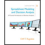
Spreadsheet Modeling & Decision Analysis: A Practical Introduction To Business Analytics, Loose-leaf Version
8th Edition
ISBN: 9781337274852
Author: Ragsdale, Cliff
Publisher: South-Western College Pub
expand_more
expand_more
format_list_bulleted
Concept explainers
Question
error_outline
This textbook solution is under construction.
Students have asked these similar questions
A careful analysis of the cost of operating an automobile was conducted by accounting manager Dia Bandaly. The following model was
developed:
y = 3,600+ 0.16x,
where y is the annual cost and x is the miles driven.
a) If the car is driven 15,000 miles this year, the forecasted cost of operating this automobile = $
b) If the car is driven 26,000 miles this year, the forecasted cost of operating this automobile = $
(enter your response as a whole number).
What price do farmers get for their watermelon crops? In the third week of July, a random sample of 42 farming regions gave a sample mean of = $6.88 per 100 pounds of watermelon. Assume that σ is known to be $1.92 per 100 pounds.
(a)
Find a 90% confidence interval for the population mean price (per 100 pounds) that farmers in this region get for their watermelon crop (in dollars). What is the margin of error (in dollars)? (For each answer, enter a number. Round your answers to two decimal places.)lower limit $ upper limit $ margin of error $
(b)
Find the sample size necessary for a 90% confidence level with maximal error of estimate E = 0.27 for the mean price per 100 pounds of watermelon. (Enter a number. Round up to the nearest whole number.) farming regions
(c)
A farm brings 15 tons of watermelon to market. Find a 90% confidence interval for the population mean cash value of this crop (in dollars). What is the margin of error (in dollars)? Hint: 1 ton is 2000…
List down the most important types of probability distributions used in quality management?
Knowledge Booster
Learn more about
Need a deep-dive on the concept behind this application? Look no further. Learn more about this topic, management and related others by exploring similar questions and additional content below.Similar questions
- Play Things is developing a new Lady Gaga doll. The company has made the following assumptions: The doll will sell for a random number of years from 1 to 10. Each of these 10 possibilities is equally likely. At the beginning of year 1, the potential market for the doll is two million. The potential market grows by an average of 4% per year. The company is 95% sure that the growth in the potential market during any year will be between 2.5% and 5.5%. It uses a normal distribution to model this. The company believes its share of the potential market during year 1 will be at worst 30%, most likely 50%, and at best 60%. It uses a triangular distribution to model this. The variable cost of producing a doll during year 1 has a triangular distribution with parameters 15, 17, and 20. The current selling price is 45. Each year, the variable cost of producing the doll will increase by an amount that is triangularly distributed with parameters 2.5%, 3%, and 3.5%. You can assume that once this change is generated, it will be the same for each year. You can also assume that the company will change its selling price by the same percentage each year. The fixed cost of developing the doll (which is incurred right away, at time 0) has a triangular distribution with parameters 5 million, 7.5 million, and 12 million. Right now there is one competitor in the market. During each year that begins with four or fewer competitors, there is a 25% chance that a new competitor will enter the market. Year t sales (for t 1) are determined as follows. Suppose that at the end of year t 1, n competitors are present (including Play Things). Then during year t, a fraction 0.9 0.1n of the company's loyal customers (last year's purchasers) will buy a doll from Play Things this year, and a fraction 0.2 0.04n of customers currently in the market ho did not purchase a doll last year will purchase a doll from Play Things this year. Adding these two provides the mean sales for this year. Then the actual sales this year is normally distributed with this mean and standard deviation equal to 7.5% of the mean. a. Use @RISK to estimate the expected NPV of this project. b. Use the percentiles in @ RISKs output to find an interval such that you are 95% certain that the companys actual NPV will be within this interval.arrow_forwardThe Baker Company wants to develop a budget to predict how overhead costs vary with activity levels. Management is trying to decide whether direct labor hours (DLH) or units produced is the better measure of activity for the firm. Monthly data for the preceding 24 months appear in the file P13_40.xlsx. Use regression analysis to determine which measure, DLH or Units (or both), should be used for the budget. How would the regression equation be used to obtain the budget for the firms overhead costs?arrow_forwardSoftware development is an inherently risky and uncertain process. For example, there are many examples of software that couldnt be finished by the scheduled release datebugs still remained and features werent ready. (Many people believe this was the case with Office 2007.) How might you simulate the development of a software product? What random inputs would be required? Which outputs would be of interest? Which measures of the probability distributions of these outputs would be most important?arrow_forward
- Based on Babich (1992). Suppose that each week each of 300 families buys a gallon of orange juice from company A, B, or C. Let pA denote the probability that a gallon produced by company A is of unsatisfactory quality, and define pB and pC similarly for companies B and C. If the last gallon of juice purchased by a family is satisfactory, the next week they will purchase a gallon of juice from the same company. If the last gallon of juice purchased by a family is not satisfactory, the family will purchase a gallon from a competitor. Consider a week in which A families have purchased juice A, B families have purchased juice B, and C families have purchased juice C. Assume that families that switch brands during a period are allocated to the remaining brands in a manner that is proportional to the current market shares of the other brands. For example, if a customer switches from brand A, there is probability B/(B + C) that he will switch to brand B and probability C/(B + C) that he will switch to brand C. Suppose that the market is currently divided equally: 10,000 families for each of the three brands. a. After a year, what will the market share for each firm be? Assume pA = 0.10, pB = 0.15, and pC = 0.20. (Hint: You will need to use the RISKBINOMLAL function to see how many people switch from A and then use the RISKBENOMIAL function again to see how many switch from A to B and from A to C. However, if your model requires more RISKBINOMIAL functions than the number allowed in the academic version of @RISK, remember that you can instead use the BENOM.INV (or the old CRITBENOM) function to generate binomially distributed random numbers. This takes the form =BINOM.INV (ntrials, psuccess, RAND()).) b. Suppose a 1% increase in market share is worth 10,000 per week to company A. Company A believes that for a cost of 1 million per year it can cut the percentage of unsatisfactory juice cartons in half. Is this worthwhile? (Use the same values of pA, pB, and pC as in part a.)arrow_forwardAn automobile manufacturer is considering whether to introduce a new model called the Racer. The profitability of the Racer depends on the following factors: The fixed cost of developing the Racer is triangularly distributed with parameters 3, 4, and 5, all in billions. Year 1 sales are normally distributed with mean 200,000 and standard deviation 50,000. Year 2 sales are normally distributed with mean equal to actual year 1 sales and standard deviation 50,000. Year 3 sales are normally distributed with mean equal to actual year 2 sales and standard deviation 50,000. The selling price in year 1 is 25,000. The year 2 selling price will be 1.05[year 1 price + 50 (% diff1)] where % diff1 is the number of percentage points by which actual year 1 sales differ from expected year 1 sales. The 1.05 factor accounts for inflation. For example, if the year 1 sales figure is 180,000, which is 10 percentage points below the expected year 1 sales, then the year 2 price will be 1.05[25,000 + 50( 10)] = 25,725. Similarly, the year 3 price will be 1.05[year 2 price + 50(% diff2)] where % diff2 is the percentage by which actual year 2 sales differ from expected year 2 sales. The variable cost in year 1 is triangularly distributed with parameters 10,000, 12,000, and 15,000, and it is assumed to increase by 5% each year. Your goal is to estimate the NPV of the new car during its first three years. Assume that the company is able to produce exactly as many cars as it can sell. Also, assume that cash flows are discounted at 10%. Simulate 1000 trials to estimate the mean and standard deviation of the NPV for the first three years of sales. Also, determine an interval such that you are 95% certain that the NPV of the Racer during its first three years of operation will be within this interval.arrow_forwardYou now have 10,000, all of which is invested in a sports team. Each year there is a 60% chance that the value of the team will increase by 60% and a 40% chance that the value of the team will decrease by 60%. Estimate the mean and median value of your investment after 50 years. Explain the large difference between the estimated mean and median.arrow_forward
- It costs a pharmaceutical company 75,000 to produce a 1000-pound batch of a drug. The average yield from a batch is unknown but the best case is 90% yield (that is, 900 pounds of good drug will be produced), the most likely case is 85% yield, and the worst case is 70% yield. The annual demand for the drug is unknown, with the best case being 20,000 pounds, the most likely case 17,500 pounds, and the worst case 10,000 pounds. The drug sells for 125 per pound and leftover amounts of the drug can be sold for 30 per pound. To maximize annual expected profit, how many batches of the drug should the company produce? You can assume that it will produce the batches only once, before demand for the drug is known.arrow_forwardYou are considering a 10-year investment project. At present, the expected cash flow each year is 10,000. Suppose, however, that each years cash flow is normally distributed with mean equal to last years actual cash flow and standard deviation 1000. For example, suppose that the actual cash flow in year 1 is 12,000. Then year 2 cash flow is normal with mean 12,000 and standard deviation 1000. Also, at the end of year 1, your best guess is that each later years expected cash flow will be 12,000. a. Estimate the mean and standard deviation of the NPV of this project. Assume that cash flows are discounted at a rate of 10% per year. b. Now assume that the project has an abandonment option. At the end of each year you can abandon the project for the value given in the file P11_60.xlsx. For example, suppose that year 1 cash flow is 4000. Then at the end of year 1, you expect cash flow for each remaining year to be 4000. This has an NPV of less than 62,000, so you should abandon the project and collect 62,000 at the end of year 1. Estimate the mean and standard deviation of the project with the abandonment option. How much would you pay for the abandonment option? (Hint: You can abandon a project at most once. So in year 5, for example, you abandon only if the sum of future expected NPVs is less than the year 5 abandonment value and the project has not yet been abandoned. Also, once you abandon the project, the actual cash flows for future years are zero. So in this case the future cash flows after abandonment should be zero in your model.)arrow_forwardThe CEO of Coral Gables Corp. was reviewing the returns of the company's sizeable investment portfolio in the last five years during a period of extreme volatility. He noted the 5 year sequence of investment returns as follows: +30%, -20%, +30%, -20%, +30%. He then calculated the arithmetic average return, but his CFO noted that since he had ignored the compounding effect he was wrong. By how much was he wrong? (Hint: Calculate the annual arithmetic average return over the five years less the average geometric (compounded) return.) (Round intermediate calculation to 2 decimal places, e.g. 52.75.) O 1.59% O 3.25% ○ 2.95% ○ 9.39%arrow_forward
- A salesperson uses three different airlines. The probabilities of switching from one airline to another in consecutive flights are shown below. If the last flight was on Delta, what is the probability that the next was on American? American Delta Southwest American 0.5 0.25 0.25 Delta 0.2 0.6 0.2 Southwest 0.3 0.3 0.4 A 0.5 B 0.2 C 0.25 D 0.6arrow_forwardThis type of analysis is most appropriate when the past is a good predictor of the future.arrow_forwardCost Estimation; High-Low and Regression Methods The Mac Davis Company specializesin the purchase, renovation, and resale of older homes. Mac employs several carpenters and paintersto do the work for him. It is essential for him to have accurate cost estimates so he can determinetotal renovation costs before he purchases a piece of property. If estimated renovation costs plus thepurchase price of a house are higher than the house’s estimated resale value, it is not a worthwhileinvestment.Mac has been using the home’s interior square feet for his exterior paint cost estimations. Recentlyhe decided to include the number of external openings—the total number of doors and windows ina house—as a cost driver. Their cost is significant because they require time-consuming preparatorywork and careful brushwork. The rest of the house usually is painted either by rollers or spray guns,which are relatively efficient ways to apply paint to a large area. Mac has kept careful records of theseexterior…arrow_forward
arrow_back_ios
SEE MORE QUESTIONS
arrow_forward_ios
Recommended textbooks for you
- Practical Management ScienceOperations ManagementISBN:9781337406659Author:WINSTON, Wayne L.Publisher:Cengage,
Practical Management Science
Operations Management
ISBN:9781337406659
Author:WINSTON, Wayne L.
Publisher:Cengage,
Inventory Management | Concepts, Examples and Solved Problems; Author: Dr. Bharatendra Rai;https://www.youtube.com/watch?v=2n9NLZTIlz8;License: Standard YouTube License, CC-BY