Chapter 10, Problem 1CRE

In Exercises 1–3, use the following service times (in seconds) observed at lunchtime at different fast-food restaurant drive-up windows. Assume that the service times for such restaurants are normally distributed.

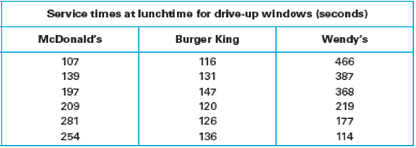
1. 1. McDonald’s. Using only the service times from McDonald’s, construct a 95% confidence interval estimate of the population mean.

To determine

Using the service times from McDonald’s obtain a 95% confidence interval to estimate the populations mean.

Answer to Problem 1CRE

The 95% confidence interval to estimate the population mean is $\left(128.37,267.29\right)$.

Explanation of Solution

Calculation:

The data related to the service times at lunchtime for drive-up windows at McDonald’s.

t-distribution:

A random variable X is said to follow t distribution with degrees of freedom $n–1$, if the probability density function of X is defined as,

$f\left(x\right)=\frac{{\left(1+\frac{x^2}{n-1}\right)}^{-\frac{n}{1}}\Gamma \left(\frac{n}{2}\right)}{\sqrt{\left(n-1\right)\pi }\Gamma \left(\frac{n-1}{2}\right)},-\infty <x<\infty$ for n observations.

The value of random variable X can be defined as,

$x=\frac{y}{\sqrt{\frac{z}{k}}}$, where the random variable y follows standard normal distribution and the random variable z follows chi-square distribution with degrees of freedom k.

Test statistic:

The test statistic is obtained as,

$t=\frac{\overline{x}-\mu }{\frac{s}{\sqrt{n}}}$, where $\overline{x}$ is the sample mean, $\mu$ is the population mean and s is the sample standard deviation.

Level of significance:

The level of significance is $\alpha =0.05$.

For two tail test the level of significance is,

$\begin{array}{c}\frac{\alpha }{2}=\frac{0.05}{2}\\ =0.025\end{array}$ .

The sample size is $n=6$.

Degrees of freedom:

The degrees of freedom for t distribution is $n-1$.

Hence, the degrees of freedom for $n=6$ is,

$\begin{array}{c}\text{df}=n-1\\ =6-1\\ =5\end{array}$

Critical value:

Step by step procedure to obtain the critical value from the TABLE 10.1: Critical t values, is obtained as:

• Locate the degrees of freedom of 5 from the 1^st column of TABLE 10.1.
• Locate the area from the column of “0.05 area in two tails” corresponding to the degrees of freedom of 5.

The critical value is 2.571.

Mean:

Software procedure:

Step by step procedure using EXCEL to obtain Mean is given below:

• Enter the name McDonald’s in the first cell A1 of an EXCEL sheet.
• Enter the data value in that sheet corresponding to the heading McDonald’s from cell A2 to A7.
• In cell A8 enter the formula “=AVERAGE(A2:A7)”.
• Click Enter.

The output is given below:

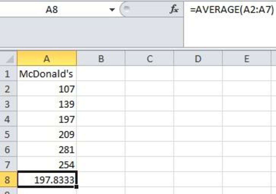
Thus, the sample mean $\overline{x}$ is approximately 197.83.

Standard deviation:

Software procedure:

Step by step procedure using EXCEL to obtain Standard deviation is given below:

• Enter the name McDonald’s in the first cell A1 of an EXCEL sheet.
• Enter the data value in that sheet corresponding to the heading McDonald’s from cell A2 to A7.
• In cell A8 enter the formula “=STDEVA(A2:A7)”.
• Click Enter.

The output is given below:

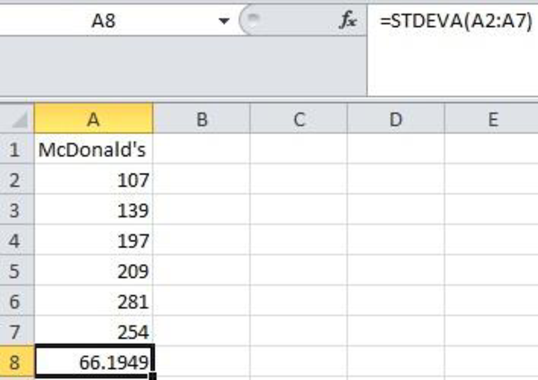
Thus, the sample standard deviation $s$ is approximately 66.19.

Margin of error:

The margin of error, E is defined as,

$E=\frac{t\times s}{\sqrt{n}}$, where t represents the critical value corresponding to the level of significance of 0.05 and s is the sample standard deviation.

The critical value is obtained as 2.571, the sample standard deviation is $s=66.19$ and sample size $n=6$.

Thus, the margin of error is,

$\begin{array}{c}E=\frac{\left(2.571\right)\left(66.19\right)}{\sqrt{6}}\\ =\frac{170.1745}{2.45}\\ \approx 69.46\end{array}$

Therefore, the margin of error is approximately 69.46

Confidence interval:

The 95% confidence interval around a sample mean to estimate the true value of population mean, $\mu$, is obtained as, $\overline{x}-E<\mu <\overline{x}+E$.

Hence the confidence interval is,

$\begin{array}{c}\left(\overline{x}\pm E\right)=\left(197.83-69.46,197.83+69.46\right)\\ =\left(128.37,267.29\right)\end{array}$

Thus, the 95% confidence interval to estimate the population mean is $\left(128.37,267.29\right)$.